Economic temperature functions

There has been something that has bothered me about the temperature function in the partition function approach last used here [1]: $f(\ell) = \log \ell < 0$ for $\ell < 1$ (or in the original application [2] in terms of money supply $m$). Typically the labor supply $\ell$ is large (millions of people employed), so this isn't a big deal. However it is possible for the "temperature" to go negative, which is a theoretical problem for small $\ell$. In thermodynamics, the analogous function is $f(T) = 1/T$, which is always positive.

Therefore I tried a different function $f(\ell) = \log (\ell + 1)$ (solid) which stays positive and approaches the original function (dashed) for $\ell \gg 1$:

The impact was fairly small on the results of [1] -- the largest difference comes in the ensemble average productivity $\langle p \rangle$ (right/second is from [1], left/first is new calculation):

There was negligible impact on the other results -- the unemployment rate even showed a slight improvement (first is new calculation, second is from [1]):

Overall, a minor impact empirically, but fairly important theoretically.

...

Update 22 September 2016

I should note that if $A \rightleftarrows L$ with IT index $p$, we have

$$
A = A_{ref} \left( \frac{L}{L_{ref}} \right)^{p}
$$

If $L \equiv L_{ref} + \ell$, then we can rewrite the previous statement as

$$
A \sim \exp \left( p \log (\ell + 1) \right)
$$

so that the original motivation for the partition function (in [2] above) would tell us that $f(\ell) = \log (\ell + 1)$.

Scopes and scales: the present value formula

I'm not entirely sure if this conversation broke off from the discussion of NGDP futures markets, but Nick Rowe put up a post about the difficulties of calculating the present value of currency. This represents another good example of why you need to be careful about scales and scope.

The basic present value formula of a coupon $C$ with interest rate $r$ at time $T$ is

$$
PV(C, r, T) = \frac{C}{(1 + r)^{T}}
$$

First, note that an interest rate is actually a time scale. The units of $r$ are percent per time period, e.g. percent per annum. Therefore we can rewrite $r$ as a time scale $r = 1/\tau$ where $\tau$ has units of time (representing, say, the e-folding time if you think about continuous compounding).

Second, this formula comes from looking at a finite non-zero interest rate over a finite period of time. You can see this because the formula breaks if you decide to take $T$ or $\tau$ to infinity in a different order:

Paul Romer had this problem with Robert Lucas: the limit doesn't converge uniformly. Romer would call taking the limits as $r = 1/\tau \rightarrow 0$ and $T \rightarrow \infty$ in a particular order "mathiness". And I think mathiness here is an indicator that you need to worry about scope. Just think about it -- why would you calculate the "present value" of coupon that had a zero interest rate? It's like figuring out how many stable nuclei decay (see previous link).

The present value formula does not apply to a zero interest rate coupon. It is out of scope.

There are only two sensible limits of the present value formula: $T/\tau = r T \gg 1$ and $T/\tau = r T \ll 1$. This means either $T \rightarrow \infty$ or $\tau \rightarrow \infty$ -- not both. If you want to take both to infinity at the same time, you have to introduce another parameter $a$ because then you can let $T = \tau/a$ and take the limit

$$
\lim_{T \rightarrow \infty} \frac{C}{(1 + a/T)^{T}} = C e^{-a}
$$

The present value can be anything between $C$ and zero. You could introduce other models for $T = T(\tau)$, but that's the point: the present value becomes model dependent. (That's what Nick Rowe does to resolve this "paradox" -- effectively introducing some combination of nominal growth and inflation.)

That also brings up another point: the present value formula doesn't have any explicit model dependence, but it does have an implicit model dependence! It critically depends on being near a macroeconomic equilibrium (David Glasner's macrofoundations). For example, it's possible the value of a corporate bond is closer to zero because there's going to be a major recession where the company defaults. Correlated plans fail to be simultaneously viable, and someone has to take a haircut.

Basically, the scope of the present value formula is near a macroeconomic equilibrium and non-zero interest rates.

The driving equilibrium

FRED has updated the data on the number of vehicle miles driven, and it looked to me like a perfect candidate for a "growth equilibrium state" analysis using minimum entropy like I did for unemployment (see that post for more details about the process). Here is the original data:

The growth rate bins (note this is not a log-linear graph, so these are not exponential growth rates, but rather linear growth rates) look something like this:

The slope that minimizes the entropy is about α = 0.062 Mmi/y ("dr" is the data list and "DR" is an interpolating function of the data list):

And here is the minimized entropy distribution (i.e. the "spikiest" distribution):

Subtracting that trend and fitting a series of logistic functions (Fermi-Dirac distributions) to the data gives a pretty good fit:

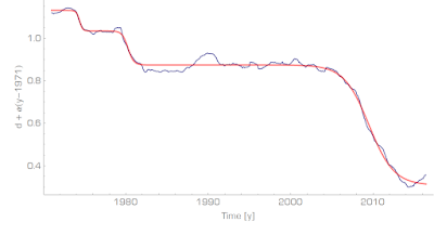
The center of the transitions are at 1974.4, 1980.3, and 2009.5 -- corresponding to the three longest recessions between 1971 and 2016. This results in a pretty good "model" of the number of vehicle miles traveled:

The monetary base continues to fall

The monetary base is continuing its slow fall; I haven't updated this graph in awhile. But first the caveat from that post:

This is probably a sucky prediction anyway since there are only about 6 data points from after the rate hike and the noise (error) has been growing over time. The symmetry argument [that the fall will be at the same rate/curvature as the rise] is doing quite a bit of work here.

Anyway, it's not really too bad ...

It's within the 2-sigma error bands ...

RGDP and employment equilibria

When I used this estimate of the "macroeconomic information equilibrium" (MIE) to claim that the mid-2000s were a "bubble" (i.e. RGDP was above the MIE), John Handley asked me what the counterfactual employment would be. Let's start with the MIE (gray) versus data (red) and "potential RGDP" from the CBO (via FRED) (black) from this post [1]:

The red line is above the gray line from rouhgly 2004 to 2008 -- that's the "bubble". We can use the information equilibrium relationship P : NGDP ⇄ EMP (EMP = PAYEMS on FRED, total non-farm employees) to say the growth rate of RGDP = NGDP/P is proportional to the growth rate of EMP; therefore the growth rate of the MIE should be the equilibrium growth rate of employment. And it is:

In [1], I noted that the information equilibrium unemployment result was a relationship between the growth rates of employment and MIE RGDP (shown in the picture above) rather than the output gap level and the unemployment rate. Basically, in the information equilibrium model

$$
\text{(1) }\; \frac{d}{dt} \log U = \left( b + a \frac{d}{dt} \log RGDP_{MIE} \right) - \frac{d}{dt} \log EMP
$$

rather than

$$
\text{(2) }\; U = b + a (RGDP - RGDP_{P})
$$

Both of these relationships work pretty well:

However, the derivative in equation (1) basically tells us that we measure the unemployment rate relative to some constant value in the IE model, but we have no idea what that value is -- it's the constant of integration you get from from integrating equation (1) -- but it also doesn't matter. Choose an arbitrary level of unemployment and then we'd say unemployment is "low" or "high" relative to that level. It is similar to the case of temperature -- 200 Kelvin is "cold", but 200 Celsius is "hot" because of the choice of zero point. Picking the average (5.9%) is as good a choice as any:

And so -- unemployment was low during the mid-2000s (well, falling since we are talking about rates). The eras where RGDP grows parallel to the MIE are also "equilibria" where unemployment is "normal" -- early 1960s; late 80s to 1990; the mid-90s; 2001-2004.

As a side note, I'd like to refer back to this post [2] which looked at unemployment equilibria in terms of the rate of decline of unemployment (rate of growth of employment). You can see how this picture basically conforms with the picture above -- the MIE is an equilibrium of growth rates, not levels. Re-fitting the data to the cases of positive employment growth in the figure above, we get this picture:

There is an employment growth equilibrium (blue line) and negative deviations (i.e. a plucking model), which is exactly the model of [2] -- unemployment decline equilibrium and unemployment increases. The model of [2] can be considered to be the approximation to the model here for constant MIE RGDP growth (i.e. unemployment declines of constant slope -- figure below from [2]).

...

Update 22 July 2016

I was a bit premature in the paragraph above after the pair of images that you couldn't figure out a reasonable employment level. It's still a "fit" since the constant of integration information is unavailable, but it doesn't mean you can't create a "zero" for the temperature scale. Here is the employment level where I fit the constant of integration to the data:

You can still shift this curve up and down, but in the same way as you refer to temperature being high or low relative to a scale (absolute zero or water freezing) you can refer to employment being high or low relative to this curve regardless of whether you shift it up or down.

Information equilibrium in neuroscience

Todd Zorick and I wrote a neuroscience paper on using information equilibrium to tell the difference between different sleep states with EEG data. The title is "Generalized Information Equilibrium Approaches to EEG Sleep Stage Discrimination" and it was (finally) published today.

This adds to the series of information equilibrium framework applications for complex systems like traffic or simple systems like transistors.

One can think of these distributions as ensembles of "information transfer states" analogous to productivity states, profit states (below), or growth states.

An ensemble of labor markets

Believe it or not, this post is actually a response of sorts to David Glasner's nice post "What's Wrong with Econ 101" and related to John Handley's request on Twitter for a computation of the implied unemployment rate given an output gap (which I will answer more directly as soon as I find the code that generated the original graph in question). It is also a "new" model, but still fairly stylized. I will start with the partition function approach described in the paper as well as here. However instead of being written in terms of money, I will write it in terms of labor.

Consider aggregate demand as a set of markets with demand $A = \{ a_{i} \}$, labor supply $L = \{ \ell_{i} \}$, information transfer indices (which I will label 'productivity states' for reasons that will become clear later) $p = \{ p_{i} \}$, and a price level $CPI = \{ cpi_{i} \}$. I use the notation:

$$
cpi_{i} : a_{i} \rightleftarrows \ell_{i}
$$

which just represents the differential equation (information equilibrium condition)

$$
cpi_{i} \equiv \frac{da_{i}}{d\ell_{i}} = p_{i} \; \frac{a_{i}}{\ell_{i}}
$$

This has solution

$$
a_{i} \sim \ell_{i}^{p_{i}}
$$

You can see how the $p_{i}$ values are related to 'productivity'; if the growth rate of $\ell_{i}$ is $r_{i}$, then the growth rate of $a_{i}$ is $p_{i} r_{i}$ and the ratio of $\ell_{i}$ to $a_{i}$ (assuming exponential growth for the two variables) is $e^{p_{i}}$.  Let's take the labor market to be a single aggregate (analogously to taking the money supply to be a single aggregate), so that we can drop the subscripts on the $\ell$'s. Define the partition function

$$
Z(\ell) \equiv \sum_{i} e^{-p_{i} \log \ell}
$$

so that the ensemble average of operator $X$ (which will be over 100 markets, i.e. $i = 1 .. 100$ with different values of $p_{i}$ in the Monte Carlo simulations below) is:

$$
\langle X \rangle = \frac{\sum_{i} X \; e^{-p_{i} \log \ell}}{Z(\ell)}
$$

I assumed the productivity states had a normal distribution which results in the following plot of 30 Monte Carlo throws for 100 markets for $\langle \ell^{p}\rangle$:

The ensemble of 'productivity states' $p_{i}$ looks something like this:

This picture illustrates David Glasner's point about general and partial equilibrium analysis in economics 101. The distribution (in black) represents a macroeconomic general equilibrium. Individual firms or markets will move from different productivity states over time. Partial equilibrium analysis looks at individual states that move or have idiosyncratic shocks that do not change the overall distribution. If the distribution changes, you have moved to a different general equilibrium and partial equilibrium analysis will not suffice. That is to say Economics 101 assumes this distribution does not change. (In this model, shocks are represented as productivity shocks, changing the values of $p_{i}$ and/or the average of the distribution in the figure.)

We can fit this ensemble average to the graph of nominal output (NGDP) versus total employees (PAYEMS on FRED, measured in Megajobs [Mj]):

The price level should then be given by the ensemble average $\langle p \ell^{p-1}\rangle$ (switching to linear scale instead of log scale):

The black lines in these graphs represent a single macroeconomic general equilibrium; as you can see, the true economy (blue) fluctuates around that equilibrium. Now the ensemble of individual markets can be represented as a single macro market, but with a (slowly) changing value of the single 'macro' information transfer index $p = \langle p_{i} \rangle$ plotted below:

Note that as the size of the labor market grows, productivity falls. This is analogous to the interpretation of the result for nominal output in terms of money supply: a large economy has more ways of being organized as many low growth states than as a few high growth ones. In thermodynamics, we'd interpret a larger economy (larger money supply or larger labor supply) as a colder economy.

The single macro market with changing $p$ is $CPI : A \rightleftarrows L$, which is basically the information equilibrium relationship that leads to Okun's law (shown in the paper as well as here in terms of hours worked, but labor supply also leads to a decent model, graph from here):

This correspondence means that we should view the difference between equilibrium output and actual output as well as the difference between the equilibrium price level and the actual price level as a measure of the output gap (difference from potential NGDP) and the unemployment rate, respectively ... which works pretty well for such a simple model:

Differences between the model and data could be interpreted as non-ideal information transfer which includes correlations among the labor markets (e.g. coordinating plans that fail together) or deviation from the equilibrium distribution of productivity states. Note that in the output gap calculation, you can see what looks like a plucking model of non-ideal information transfer with a changing equilibrium.

This simple model brings together output and employment, falling inflation and productivity, as well as macroeconomic general equilibrium and microeconomic partial equilibrium in a single coherent framework. It's not perfect empirically, but there isn't much competition out there!

...

Update 19 July 2016

Here's how the distribution of 'productivity' states changes as $\ell$ increases:

List of standard economics derived from information equilibrium

Here is a (possibly incomplete, and hopefully growing) list of standard economic results I have derived from information equilibrium. It will serve as a reference post. This does not mean these results are "correct", only that they exist given certain assumptions. For example, the quantity theory of money is only really approximately true if inflation is "high". Another way to say this is that information equilibrium includes these results of standard economics and could reduce to them in certain limits (like how quantum mechanics reduces to Newtonian physics for large objects).

In a sense, this is supposed to serve as an acknowledgement (or evidence) that information equilibrium has a connection to mainstream economics ... and that it's not completely crackpottery.

Supply and demand

http://informationtransfereconomics.blogspot.com/2013/04/supply-and-demand-from-information.html

Price elasticities

http://informationtransfereconomics.blogspot.com/2013/04/the-previous-post-with-more-words-and.html

Comparative advantage

http://informationtransfereconomics.blogspot.com/2016/04/comparative-advantage-from-maximum.html

AD-AS model

http://informationtransfereconomics.blogspot.com/2015/04/what-does-ad-as-model-mean.html

IS-LM

http://informationtransfereconomics.blogspot.com/2013/08/deriving-is-lm-model-from-information.html
http://informationtransfereconomics.blogspot.com/2014/03/the-islm-model-again.html
http://informationtransfereconomics.blogspot.com/2016/02/the-is-lm-model-as-effective-theory-at.html

Quantity theory of money

http://informationtransfereconomics.blogspot.com/2013/07/recovering-quantity-theory-from.html
http://informationtransfereconomics.blogspot.com/2015/05/money-defined-as-information-mediation.html

Cobb-Douglas functions

http://informationtransfereconomics.blogspot.com/2014/05/more-on-cobb-douglas-functions-and.html

Solow growth model

http://informationtransfereconomics.blogspot.com/2014/12/the-information-transfer-solow-growth.html
http://informationtransfereconomics.blogspot.com/2015/05/the-rest-of-solow-model.html
http://informationtransfereconomics.blogspot.com/2015/05/dynamics-of-savings-rate-and-solow-is-lm.html

The Kaldor facts as information equilibrium relationships

http://informationtransfereconomics.blogspot.com/2016/09/the-kaldor-facts.html

Gravity models

http://informationtransfereconomics.blogspot.com/2015/09/information-equilibrium-and-gravity.html

Utility maximization

http://informationtransfereconomics.blogspot.com/2015/03/utility-in-information-equilibrium-model.html

Asset pricing equation

http://informationtransfereconomics.blogspot.com/2015/05/the-basic-asset-pricing-equation-as.html

Euler equation

http://informationtransfereconomics.blogspot.com/2015/06/the-euler-equation-as-maximum-entropy.html

DSGE models

http://informationtransfereconomics.blogspot.com/2016/08/dsge-part-1.html
http://informationtransfereconomics.blogspot.com/2016/08/dsge-part-2.html
http://informationtransfereconomics.blogspot.com/2016/08/dsge-part-3-stochastic-interlude.html
http://informationtransfereconomics.blogspot.com/2016/08/dsge-part-4.html
http://informationtransfereconomics.blogspot.com/2016/08/dsge-part-5-summary.html

MINIMAC

http://informationtransfereconomics.blogspot.com/2015/06/minimac-as-information-equilibrium-model.html

Mundell-Fleming as Metzler diagram

http://informationtransfereconomics.blogspot.com/2016/06/metzler-diagrams-from-information.html

Diamond-Dybvig

http://informationtransfereconomics.blogspot.com/2015/04/diamond-dybvig-as-maximum-entropy-model.html

"Econ 101" effects of price ceilings or floors

http://informationtransfereconomics.blogspot.com/2016/05/what-happens-when-you-push-on-price.html

Cagan model

http://informationtransfereconomics.blogspot.com/2016/08/the-economy-at-end-of-universe-part-ii.html

Lucas Islands model

http://informationtransfereconomics.blogspot.com/2015/04/towards-information-equilibrium-take-on.html

"A statistical equilibrium approach to the distribution of profit rates"

That's the title of a paper [pdf] by Gregor Semieniuk (and his co-author) who tried to get a hold of me at the BPE meeting (which I was unfortunately unable to attend, but did make some slides). The paper notes that the distributions of the rates of profit appear to have invariant distributions suggestive of statistical equilibrium; here's a diagram:

This diagram is reminiscent of the diagrams I've used when talking about the distribution of growth states in an economy, most colorfully illustrated at this link (and discussed here and in my paper; note that Gregor's diagram has a log scale for the y-axis).

In fact, it might be directly related. If we have a series of markets (or firms) where income $I_{k}$ is in information equilibrium with expenses $E_{k}$ with "price" $p_{k}$, i.e. $p : I \rightleftarrows E$, in general equilibrium we have

$$
\frac{I_{k}}{I_{k, ref}} = \left( \frac{E_{k}}{E_{k, ref}}\right)^{p_{k}}
$$

so that for $E_{k} \approx E_{k, ref}$

$$
I_{k} \approx I_{k, ref} + p_{k} \frac{I_{k, ref}}{E_{k, ref}} (E_{k}-E_{k, ref})
$$

Therefore $p_{k}$ determines the rate of profit (difference between income and expenses). It determines how much bigger $I$ is given $E$. If $p = 1$, then profit is zero because income equals expenses. If $p > 1$, the firm is profitable because $I > E$; vice versa for $p < 1$. In the partition function approach (also discussed in the paper and the link above), the "prices" represent growth states; here, the "prices" represent profit states. The distribution represents an equilibrium "temperature".

We'd also expect the profit states to have some distribution around a mean value, but have negative profit states to be over-represented due to non-ideal information transfer. This is as observed in the diagram from Gregor's paper. It is also observed in nominal growth data over time** (figure from my paper linked above; also see here):

** This implies a macroeconomy is ergodic: the distribution of temporal states are the same as distributions of ensembles of states.

...

Update 01 August 2016

Michael Williams sent me links to two of his (and co-authors') papers (here and here) where they look at the distribution of economic profit rates and firm growth rates. These appear to have well-defined distributions as in the paper from Semieniuk et al above. The difference is that Williams et al find that the distributions appear to be Cauchy distributions rather than Laplace distributions. I noted previously that the distribution of wage changes also appears (by eye -- I did no rigorous testing) to be Cauchy (plus perturbations).

Laplace distributions are maximum entropy distributions subject to the constraint on the absolute deviation |Δ| = |x - μ| of the variable (profit rate in this case) from the mean. Semieniuk et al also suggest the asymmetric Laplace distribution which is the maximum entropy distribution subject to a constraint on the average deviation (Δ = x - μ).

Cauchy distributions are "heavy-tailed" and are the maximum entropy distributions for random variables subject to a constraint on log(1+Δ²) where Δ = x - x₀ (the Cauchy distribution has no mean, so there is a parameter x₀ that represents the "center").

In my view the Laplace distribution represents a "first order approximation" which is improved upon with the Cauchy distribution. However, I'd take a more agnostic view that what we have is some form of stable distribution (of which the Cauchy distribution is a particular example). Note that Mandelbrot showed that stable distributions appeared to fit various financial data. Here's a graph with a Cauchy (blue), stable (yellow), and skewed stable (green) distributions along with a Laplace distribution (gray dashed):

Stable distributions are stable in the sense that they have their own (more general) central limit theorem that doesn't require a finite variance.

Ceteris paribus and method of nascent science

I read this from Arnold Kling about models in economics:

... In economics, models are often used for a different purpose. The economist writes down a model in order to demonstrate or clarify the connection between assumptions and conclusions. The typical result is a conclusion that states 

All other things equal [ceteris paribus], if the assumptions of this model hold, then we will observe that when X happens, Y happens. 

... However, suppose that we observe a situation where X happens and Y does not happen. Does that refute the model? I would say that what it refutes is the prefatory clause “[all] other things equal, if the assumptions of this model hold.” That is, we may conclude that [all] other things were not equal or that the assumptions of the model do not hold.

Kling did leave off the [all] which I inserted above. This seems to be not atypical of economists' approach to models. I put up immediate thoughts on Twitter:

"Ceteris paribus" is problematic. All other influences aren't always known, so model fail due to [ceteris paribus] violation tells you exactly nothing.

This lead to discussion with Brennan Peterson (who I discovered recently was a friend of a close friend of mine I knew from grad school — small world) that brought up some good points. For example, even in natural sciences you don't necessarily know all other influences and therefore you cannot be certain you've isolated the system. Very true.

In fact, I discussed before how natural sciences got lucky in this regard:

I don't think this [summary of Dani Rodrik's view of models] could have been put in a better way to illustrate what is wrong with this view and how lucky scientists turned out to be. Our basic human intuition that effects tend not to pass through barriers and that increased distance from something diminishes its effect turned out to be right in most physical theories of the world. That is to say even without a theoretical framework for how the world worked, our intuition on what reduced the impact of extraneous influence was right. ... Scientists were able to boot-strap themselves into the theory because our physical intuitions matched up with the correct theory.

I'd add here that this is probably not an accident: we evolved (and grew up) dealing with the natural world, therefore our intuitions (and learned behavior) about the natural world should be useful [ETA: at least at our human scale! [1]]. In that post, I contrasted this with economics where not only do we not know how to isolate the system, but have we observed human cognitive biases with regard to economic decisions (money illusion, endowment effect). In macroeconomics, the idea of being able to isolate monetary policy with theory (i.e. ceteris paribus conditions) is incredibly difficult because we don't really know what that theoretical framework is. Additionally, it could well be that even microeconomic effects that we observe requires us to be near a macroeconomic equilibrium (Glasner's macrofoundations of micro) so the problems with macro infect micro as well.

If you think about it, the scientific method doesn't actually work for situations like this, and it's not just about Hume's uniformity of nature assumption and the problem of induction.

The induction problem is basically the question of whether you can turn a series of observations into a rule that holds for future observations (the temporal version — will the sun rise tomorrow?), or whether you can turn a series of observations of members of a class into a rule about the class (the "spatial" version — are all swans white?).

The basic conclusion is that you can't do this logically. From every sunrise, you cannot logically make any conclusion about the next sunrise without either 1) assuming it will because you've made observations that it happens every ~ 24 hours and that's worked out so far or 2) using a theoretical framework that has been useful for other things.

What we are talking about with economics is whether we can even define what a sunrise is because you need that theoretical framework in order to define it, but you couldn't build that framework without basing it on the empirical regularity that is the sunrise. Another way to say this is that you have a chicken or the egg problem: a theoretical framework aggregates past empirical successes, but you need the theoretical framework to understand the empirical data to determine those successes.

With the sunrise, we as humans took route of the Samuel Johnsons and told the effective George Berkeleys saying the sunrise doesn't exist that we refute it thus and pointing emphatically at the really bright thing on the horizon. (Not really, but imagine we invented philosophy and logic before religion which takes the assumption route about the sunrise mentioned above.)

With immaterialism or the problem of induction, I personally would say that "Well, logically, you could take that position ... stuff doesn't exist and you can't extrapolate from a series of sunrises ... but how does that help you? What is it good for?" And I think that's the key point in how you bootstrap yourself from blindly groping the dark for understanding to the scientific method. The scientific method needs a seed from which to start and that seed is a collection of useful facts. Not rigorous, not logical ... just useful. This could be e.g. evolutionary usefulness (survival of the species).

Let's go back to Kling's model. When it fails due to ceteris not being paribus, our lack of a theoretical framework organizing prior empirical successes containing that model, we learn exactly nothing. If the model had been inside a useful theoretical framework, then we'd have learned something about the limits of that theoretical framework. Without it we learn nothing.

We learn that "all other things equal" is false; some things weren't equal. But this doesn't tell us which things weren't equal, only they exist — completely useless information. We could then take the option of just assuming the model is true, but just not for the situation we encountered.

We should reject Kling's model not because it is rigorously and scientifically rejected by empirical data (it isn't), but because it is useless. Awhile ago, Noah Smith brought up the issue in economics that there are millions of theories and no way to reject them scientifically. And that's true! But I'm fairly sure we can reject most of them for being useless.

"Useless" is a much less rigorous and much broader category than "rejected". It also isn't necessarily a property of a single model on its own. If two independently useful models are completely different but are both consistent with the empirical data, then both models are useless. Because both models exist, they are useless. If one didn't, the other would be useful. My discussion with Brennan touched on this — specifically the saltwater/freshwater divide in macro. I'm not completely convinced this is an honest academic disagreement (it seems to be political), but let's say it is. Let's say both saltwater and freshwater macro aren't rejected by the empirical data and they both give "useful" policy advice on their own. Ok, well both models are useless because they provide different policy prescriptions and there's no way to say which one is right.

It's kind of like advice that says you could take either option you put forward. It's useless. That's basically the source of Harry Truman's quip about a one-armed economist.

Usefulness is how you bootstrap yourself into doing real science — there's a scientific method and a scientific method for nascent science. And economics should be considered a nascent science. It is qualitatively different than an established science like physics.

Physics wasn't always an established science; in the 1500s and 1600s it was nascent. The useful things were the heliocentric solar system (it was easier to calculate where planets would be, which we only really cared about for religious and astrological reasons), Galileo's understanding of projectile motion (to aim cannons), and Huygen's optics. Basically: religious and military utility. These were organized with a theoretical framework by Newton and physics as a science, not just a nascent science, started.

In medicine, we had a large collection of useful treatments (e.g. the ideas behind triage developed in the French Revolution), sterilization (pasteurization before pasteur), public health (Cholera in London) before the germ theory of disease. Medicine didn't really become  a science until the 1900s.

In economics, both macro and micro, we probably have a few of the "useful" concepts in our possession. Supply and demand. Okun's law. The quantity theory of money is probably useful in some form (though not necessarily as it exists now). We probably need a few more. I'd personally like to put forward this graph about interest rates as a potential candidate:

However, we should differentiate between nascent science and established science. Established science uses the scientific method and has a philosophy that includes things like falsifiablity (not necessarily Popper's form). Nascent sciences need much more practical — much more human-focused — metrics like usefulness.

...

Update 12 July 2016

Good comments from Tom Hickey.

...

Update 8 September 2020

[1] This famously does not include quantum effects — which are not at the human scale.