A strange phrenology of money

A section of something cool I saw at the Tate Modern yesterday that is mildly relevant. Details to follow when I have a real computer. [Here is a link; it's part of a work by Alexander Brodsky and Ilya Utkin.]

Gah! I always seem to miss the big macro debate flare ups when I'm on vacation.

So Paul Krugman called out monetarism and Scott Sumner and Nick Rowe responded (among others). I will add some links when I have access to a real computer and am not writing on my iPhone waiting to get on a bus to go Stonehenge for the winter solstice.

Summer touts his model getting e.g. the US and Australia right. Japan and Switzerland, too.

But why can't the BoJ get inflation, whereas Australia can reach NGDP targets? No, really. Why? The central banks are just organizations of humans ... If I took the BoJ and put it in charge of Australia and vice versa, would I get different results? Why? That actually implies that the specific humans in charge matter! Literally it matters that Greenspan or whoever is in charge -- the math is irrelevant, and it becomes a question similar to whether a president or general was a 'good leader'. Macroeconomics becomes a strange phrenology of money with lots of detailed equations and models that all purport to divine that ineffable quality of a "great man" (or woman) that could get the inflation target he or she wanted at any central bank.

And Nick Rowe's word games posit a central bank that "does nothing" that is massively deflationary. I don't think anyone has said that a central bank can't achieve deflation. But what really is problematic is that the definition of doing nothing is irrelevant to Japan. M(t) and m(t) both define the same path of the monetary base, both of which are increasing, and neither of which seem to affect the price level. It really doesn't matter how you word it.

However, the information transfer model shows how a Japan or an Australia can exist simultaneously in the same framework. If they traded central banks, they'd get largely the same results as they're getting now [i.e. Japan would be in a liquidity trap and Australia wouldn't]. And it shows how 'doing nothing' -- keeping a constantly increasing monetary base -- eventually leads to impotent monetary policy. And it shows how major increases in the base can have zero impact on inflation.

And the model isn't even that complicated.

[Updated 1/7/2015 with links and some bracketed comments.]

Echoes of the financial crisis

I'm procrastinating packing for my trip.

But Scott Sumner mentioned the Big Bang today, which as a physicist, gives me license to opine about the subject at hand. He says:

Instead, the recent deflation [2014] is a distinct echo of the actual NGDP “deflation” ... that occurred in the early part of this decade [2010-2011].

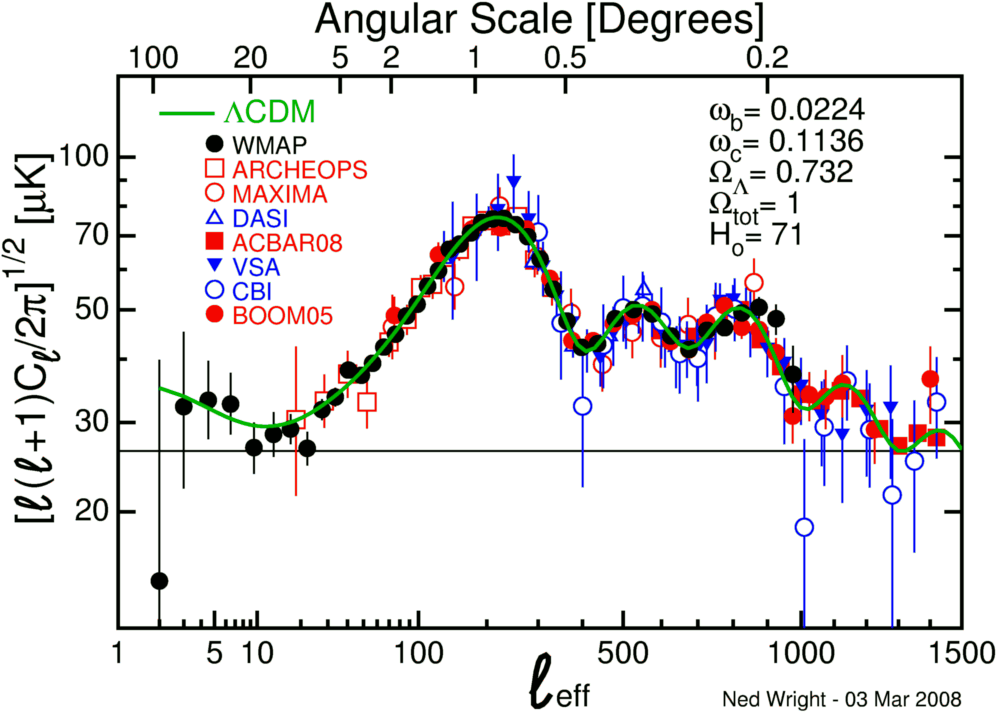
At the top of this post is the (spatial) power spectrum of the fluctuations in the cosmic microwave background (CMB) radiation. This (spatial) ringing (echo) is similar to the ringing you'll sometimes see in a jpeg image that derives from e.g. "overshooting".

Sumner's story is that earlier changes in NGDP are showing up now in inflation after being obscured by commodity prices. I'd like to put forward an alternative story using the information transfer model. The current deflation is mostly part of a long run trend, but there are fluctuations that are echoes of the real big bang: the 2008 financial crisis.

First, let's separate out the contributions to the price level from NGDP terms and monetary base terms (we can do this in the information transfer model):

There is a faint hint of a ringing from the late 2008 financial crisis. I did a fit to a simple ~ exp(t) sin(t) model for these two components:

This actually works really well. However you'd only be able to see it if you can separate out these two components because the fluctuations are almost too small to pull out in the sum relative to the magnitude of the noise. 

This model puts the source of the ringing at the financial crisis -- the commodity booms of the early part of the decade likely follow from it (basically a rebound from the low) as well as the recent deflation (which is on top of a long run trend towards deflation).

It's still not a perfect model, but it's an interesting take. Here's the graph of all the pieces together:

An information transfer traffic model

David Glasner is getting into complexity theory with his two recent posts. In the post from today he talks about traffic as a non-equilibrium complex system and quotes from a paper by Brian Arthur. In an effort to win Glasner over to an information theory view of economics, I'd like to show that a traffic system can be understood in a first order analysis with the information transfer model (or information equilibrium model). The power of the framework is demonstrated by the fact that I put this entire post together in a little over an hour on my lunch break.

Let me quote from the abstract of the paper by Fielitz and Borchardt [1] that formulates the information transfer model -- non-equilibrium complex systems is exactly what the model was designed to work with:

Information theory provides shortcuts which allow one to deal with complex systems. The basic idea one uses for this purpose is the maximum entropy principle developed by Jaynes. However, an extension of this maximum entropy principle to systems far from thermodynamic equilibrium or even to non-physical systems is problematic because it requires an adequate choice of constraints. In this paper we discuss a general concept of natural information equilibrium which does not require any choice of adequate constraints. It is, therefore, directly applicable to systems far from thermodynamic equilibrium and to non-physical systems/processes (e.g. biological processes and economical processes).

[Fielitz and Borchardt added the "economical" after learning of my blog and we periodically discuss how to properly interpret the model for economics. They have been a valuable resource in my research on this subject.]

We will set up the model as a set of distance slots (X) transferring information to a set of time (T) slots -- these become our process variables (see the preceding diagram). [Another way, X is in information equilibrium with T.] The other key ingredient is the "detector", a differential relationship between the process variables that detects information transfer [or changes in equilibrium], which we identify as the velocity:

$$
V = \frac{dX}{dT}
$$

If we assume that the information transfer is ideal so that the information in the distribution of the occupation over the distance slots is equal to the information in the distribution over the time slots, i.e. $I(T) = I(X)$

We can use the theory [1] to state:

$$
\text{(1) } V = \frac{dX}{dT} = \frac{1}{\kappa} \frac{X}{T}
$$

where $\kappa$ is constant (if the slots in the diagram above don't change) that can be worked out from theory, but can also be taken from empirical observations. It's called the information transfer index. This equation represents an abstract diffusion process [1] and we have

$$
(X)^{2} \sim (T)^{2 \kappa}
$$

And for $\kappa = 1/2$, you recover Fick's law of diffusion. However other relationships are allowed (sub- and super-diffusion) for different values of $\kappa$. It accounts for e.g. the number of lanes or the speed limits [or number of vehicles]. This is the equilibrium model of Arthur:

A typical model would acknowledge that at close separation from cars in front, cars lower their speed, and at wide separation they raise it. A given high density of traffic of N cars per mile would imply a certain average separation, and cars would slow or accelerate to a speed that corresponds. Trivially, an equilibrium speed emerges, and if we were restricting solutions to equilibrium that is all we would see.

Additionally, "supply and demand" curves follow from the equation (1) for movements near equilibrium. The "demand curve" is the distance curve and the "supply curve" is the time curve. Some simple relationships follow: an increase in time means a fall in speed at constant distance (increase in supply means a fall in price at constant demand), and an increase in distance results in an increase in speed at constant time. These are not necessarily useful for traffic, but are far more valuable for economics. The parameter $\kappa$ effectively sets the price elasticities.

However, if we look at non-ideal information transfer we have $I(T) \leq I(X)$ and equation (1) becomes

$$
V = \frac{dX}{dT} \leq \frac{1}{\kappa} \frac{X}{T}
$$

In this case the velocity falls below the ideal equilibrium price. Glasner continues his quote of Arthur

But in practice at high density, a non-equilibrium phenomenon occurs. Some car may slow down — its driver may lose concentration or get distracted — and this might cause cars behind to slow down.

Our model produces something akin to Milton Friedman's plucking model where there is a level given by the theory and then the "price" (velocity) falls below that level during recessions (traffic jams):

The key to the slowdown is coordination [2]. When there is no traffic jam, drivers drive at some speed that has e.g. a normal distribution centered near the speed limit -- their speeds are uncoordinated with each other (just coordinated with the speed limit -- the drivers' speeds represent independent samples). For whatever reason (construction, an accident, too many cars on the road), drivers velocities become coordinated -- they slow down together. This coordination can be associated with a loss of entropy [2] as drivers' velocities are no longer normally distributed near the speed limit but become coordinated in a slow crawl.

This isn't a complete model -- it is more like a first order analysis. It allows you to extract trends and can be used to e.g. guide the development of a theory for how coordinations happen based on microfoundations like reaction times and following distances. In a sense, the information transfer model might be the macrofoundations necessary to study the microeconomic model.

For the information transfer model of economics, one just has to change $X$ to NGDP, $T$ to the monetary base, and $V$ to the price level. There's also an application to interest rates and employment. As a special aside, Okun's law drops out of this framework with just a few lines of algebra.

Also, the speed limit can coordinate the distribution of velocities -- much like the central bank can coordinate expectations. I'd also like to note that no matter what the speed limit is, the speed of the traffic may not reach that because there are too many cars. This may be an analogy for e.g. Japan, the US and the EU undershooting their inflation targets.

And finally, there may be two complementary interpretations of this framework for economics. One as demand transferring information to the supply via the market mechanism and another as the future allocation of goods and services transferring information to the present allocation via the market mechanism.

[1] http://arxiv.org/abs/0905.0610
[2] http://informationtransfereconomics.blogspot.com/2014/10/coordination-costs-money-causes.html

On travel for fun for once

There's going to be a long pause on the blog. I'm going to be on vacation through the beginning of January 2015 -- I'm headed to the UK for a little over three weeks. Mostly in London and then up to Scotland for a bit. I've never been to the UK; if anyone has any travel tips, feel free to leave them in comments. Restaurant recommendations in London (we'll be staying in Pimlico) or Edinburgh are very welcome -- especially kid-friendly places.

When I get back, I'd like to start off the new year with how the predictions I've made with the information transfer model are coming along. I'm also considering switching over from Mathematica to iPython in order to more readily distribute source code to those that are interested.

And don't forget: 2015 is supposed to be the year information theory starts to have an influence on macroeconomics.

Many thanks for reading, and have a happy new year!

Inflation is information theory not ethical philiosophy

Scott Sumner argues that there has been both zero inflation and that 100% of NGDP growth was inflation (both since 1964). Tyler Cowen makes a good point about these arguments changing with income. However, Sumner's main conclusion is that inflation is a pointless concept -- in terms of understanding macroeconomic systems.

I think the real answer here is that economists don't really know what inflation is and they fall back on 19th century concepts like utility to ground them. Cowen and Sumner both ask if you'd rather live in 1964 or 2014 with a given nominal income. If that's what defines inflation -- hedonic adjustments and utility -- then I'd totally agree with Sumner: that's pointless.

But it is in this arena that the information transfer model may provide its most important insight (regardless of whether you picture money as transferring information from demand to supply or from the future to the present). The idea is spread over two posts, with the second being the main result:

1. What is inflation?
2. Expectations (rational or otherwise) and information loss

When money (M) is added to an economy, that means more information is being moved around. The difference between how much more information could theoretically be moved around with that money (proportional to M^k) and how much more information is empirically observed to be moved around (proportional to measured NGDP) is inflation.

Inflation has nothing to do with the specific goods and services being sold at a given time. It doesn't matter whether it's an iPhone or a fancy dinner. It doesn't matter whether it's toilet paper or bacon. Inflation is an information theoretical concept, not a philosophical utilitarian one.

How money transfers information from the future to the present

Widgets and money flow from their present allocation to their new future allocation while information in the future distribution flows to the present, transferred by the exchange. Widgets and coins (isotype) are from original work by Gerd Arntz.

Continuing along this path where we re-interpret the information transfer model as a picture of information flowing from the immediate future to the present through exchange. The diagram at the top of this post is meant to be a re-interpretation of the diagrams from this post.

Overall, this does not represent a mathematical difference, but rather a conceptual difference. Instead of organizing supply and demand "spatially" we're organizing it "temporally". This way of thinking about the process does help with the question of which way the information flows. There have been a few comments on this blog and elsewhere questioning how we know the information flows from the demand to the supply. In this way of picturing the model, information flows from the future to the present through market exchanges (the market is figuring out the future allocation of goods and money and uncovering that distribution means information is flowing from the future to the present).

This picture also gives us a new way to think about "aggregate demand": it derives from the allocation of goods and services in the future.

The information transfer model (information equilibrium) can also be stated more clearly using this picture. The ITM equates the information flowing from the future to the present though money to the information flowing from the future to the present through the goods. Of course you could always re-arrange this and say that the amount of information sent by the demand is equal to the amount of information received by the supply. However, I think the former description is much clearer.

The total amount of information that flows from the future to the present (in a given period of time) could be measured by e.g. the KL divergence between the future and present allocations. Since our knowledge of the future is imperfect, our expectations of the future allocation represent a loss of information, and this representation gives us a framework to start talking about that more explicitly.

Meeting expectations halfway

 

Proceeding in the spirit that theories that are correct have several different formulations, and in conjunction with my fever-dream post from yesterday, I thought I'd start a project where I re-interpret the information transfer model in terms of expectations. Maybe it will lead nowhere. Maybe this is how I should have started. I've tried to make contact with macro theories that contain expectations before, but my general attitude is that "expectations" terms as components in a model are unconstrained and allow you to get any result you'd like.

But maybe that is a strength? If potential expectations are unconstrained, then they could be anything -- and we can simply assume complete ignorance about the expectations that produce a given macrostate (i.e. all expectations microstates consistent with the macrostate defined by NGDP, inflation, interest rates, etc are equally probable).

Let's go back to the original model and instead of calling the information source "the demand" and the destination "the supply" let's set it up as a system where information about an expected future is received by the present via the market mechanism. Our diagram is at the top of this post. From there, everything else on this blog follows through essentially with a re-labeling of demand as "expected demand".

I will do a couple of short posts as I think about the implications of this idea in terms of previous results. If this concept triggers any flashes of insight from anyone out there, let me know in comments. My initial feeling is that these expectations are unlike anything economists currently think of as expectations. A central bank still cannot target an inflation rate over the long run. In the normal formulation, if the central bank sets a target, expectations should anchor on that target. There is no reason for these expectations in the theory in the diagram to anchor on some other number. But maybe the undershooting in inflation is a sign that some information is being lost?

I don't know the answers and maybe this will lead nowhere, but I thought this is a more coherent description of what I was going for in my previous post.

What does $E_{t} \pi_{t+1}$ mean?

Figure from NY Fed [pdf] modified using excerpts from Lena Nyadbi's dayiwul lirlmim barramundi.

Sorry for the $\LaTeX$ in the title but I'm currently trying to decipher some DSGE models and there is a lack of a clear answer in various economics papers as to what e.g. the term

$$
E_{t} \pi_{t+1}
$$

means. The best answer comes from here [pdf]:

The expectations are typically modeled as being formed according to the rational expectations hypothesis. The notation $E_{t}$ in the model denotes model-consistent rational expectations, i.e., the mathematical conditional expectation based on time-t information set and derived from the model ... itself.

So if we assume rational expectations we basically come to the conclusion:

$$
E_{t} \pi_{t+1} = \pi_{t+1}
$$

Are economists embarrassed to have terms from the future in their equations so they invent a new notation that says "oh, no, this term isn't really future inflation in our model that's trying to predict the future"? Now that's a bit uncharitable and this is really (where the vertical bar means evaluated with/at)

$$
E_{t} \pi_{t+1} = \pi_{t+1} \vert_{\sigma^{i}_{t+1} = 0}
$$

where $\sigma^{i}_{t+1}$ is whatever random process(es) or shocks that generate the fluctuations (in the original RBC model this is TFP). I personally like that notation because it makes the rational expectations assumption $\sigma^{i}_{t+1} = 0$ explicit. The best notation would probably be (in fact, has been used in the past)

$$
\pi^{E}_{t+1}
$$

where the $E_{t}$ represents just a label for whatever model of expectations you are using -- as there are different models of expectations besides rational expectations. For example, as best I can tell, the model independent expectations that happen in e.g. market monetarism where the central bank, if credible, can target any price level path (see e.g. Nick Rowe here) it chooses look like this

$$
E_{t} \pi_{t+1} = \Pi (t+1)
$$

where $\Pi (t)$ is a price level path function that sets the price level for each time period $t$. You could get fancy here and have the expectations follow a smooth path over more than a single time period to get back on track (mechanisms like sticky prices could slow adjustment from any given shock).

One issue with this model is that it sometimes seems to be used to go the wrong way. David Beckworth has said (paraphrasing) "Yes, the central bank may say that the price level has path $\Pi_{1} (t)$, but really it has path $\Pi_{2} (t)$" where empirical values $\pi_{t}$ are used to infer $\Pi_{2} (t)$. The specific issue with this is that a path $\Pi_{2} (t)$ that matches up with empirical data likely exists for pretty much any model. The inferred path $\Pi_{2} (t)$ becomes a universal fudge factor that instead of explaining the empirical data decouples your theory from the empirical data.

Neither of these views escape the fact that a potentially rapidly changing (and possibly counterfactual) future [1] is directly coupled to an otherwise concrete theory. Now this isn't necessarily incorrect per se -- maybe things really are that uncertain and subjective. Who knows? But it gets weirder. Let's hand the floor over to Scott Sumner:

At first glance my hypothesis [that the (future) interest rate increase of 2015 caused the Great Recession] seems absurd for many reasons, primarily because effect is not suppose to precede cause. So let me change the wording slightly, and suggest that expectations of this 2015 rate increase caused the Great Recession. Still seems like a long shot, but it's actually far more plausible than you imagine (and indeed is consistent with mainstream macro theory.)

Yes, this is totally consistent with mainstream macro -- the two equations above show how information (and changing information) about the future can potentially propagate backwards into the past. All you need to do is couple a $t+1$ term to a $t$ term. That may be why economists sheepishly write those $E_{t}$ terms.

But I have an additional critique beyond the basic structure of expectations-based macroeconomic theories that might seem a bit strange and it's related to the causality problems with Sumner's hypothesis. What keeps expectations in the future? What prevents expectations of $\pi_{t+1}$ from becoming the value of $\pi_{t}$? What keeps the dreamtime from becoming all time? [2]

In a sense, expectations can travel from a point the future to the present instantaneously -- a kind of temporal 'action at a distance' [3]. There are two things that appear to stop this in macro models:

1. Sticky prices/wages: the empirically observed fact that some prices are slow to change
2. Uncertainty: because the future is uncertain, the full impact of expectations is reduced

Interestingly, both of these ideas have interpretations in terms of entropic forces. Prices are sticky because the price distribution cannot spontaneously organize itself (destroy uncertainty information about the microstates) in a way that allows prices to change and the very definition of an entropic force is a force that serves to preserve or restore uncertainty about the microstate (increase entropy).

Can we therefore interpret the information transfer model as a model of economic dreamtime? In the information transfer model, we assume all possible microstates consistent with current macro observations are not only possible, but equally probable. That includes all possible future paths of the price level. Is modeling a macroeconomy with expectations no different than assuming you know nothing about how macroeconomics works?

With expectations, we decouple the the bulk of the DSGE model (the concrete theory) from the data. Maybe that is a good thing, and instead of the various boxes in the diagram at the top of this post and the blob of economic dreamtime expectations that includes all possible futures and the empirical data all we need is the blob (which we model by assuming ignorance of what it is) and the empirical data. The information transfer model is the model of expectations that instantly propagates expectations of the future to the present and completely dominates the concrete theory.

The spice is the worm. The worm is the spice.

[1] I like to imagine it visually as aboriginal dreamtime paintings.

[2] I think the dreamtime metaphor is especially useful here because dreamtime represents the past and future holistically.

[3] It's funny that action at a distance is associated with a violation of special relativity (the constant speed of light) which is in turn associated with causality violation.

Information equilibrium theories satisfy the Lucas critique

Image from wikimedia commons and modified by me with a random Voronoi diagram to sort of suggest Planck areas measuring the surface units of information.

Despite being annoyed by me, Noah Smith is probably one of the best blogging resources for understanding modern macroeconomics around today, and I frequently go back through his archives and click through the many self-referential links on his blog (a method I have apparently copied). This may be an educational style bias as Noah was an undergraduate physics major, giving us a common point of reference. And there is, of course, the same excellent last name.

Anyway, I was just reading this post of his on the Lucas critique -- the idea that observed macroeconomic relationships may change if you try to use them for policy (the prime example of which is the Phillips Curve which seemed to go away when it was used for policy). Noah quotes Charles Plosser:

Plosser says that "almost no model [has] satisfactorily dealt with the [Lucas Critique]."

Noah then proceeds to ask how one would satisfy the Lucas critique and identifies three methods:

• Macro experiments (in real or virtual worlds)
• Real microfoundations and detailed simulations (agent-based models)
• Vague judgment calls (which is Noah's observation of how things seem to work)

This leaves out a fourth possibility

• Assume as little as possible about the microfoundations and see how far that can take you

This fourth possibility is the the approach taken in the 19th century to understand thermodynamics (we knew little about atoms at the time), but is also behind maximum entropy methods and -- particularly relevant to this blog -- information equilibrium (such as the information transfer model). Note that I've talked about this before in relation to the Lucas critique.

I'm not sure I've made this clear enough on this blog, but in a sense, whatever theory of macroeconomics turns out to be correct, the information transfer model has to be correct. Note that I've talked about this before as well.

The information transfer model may not be useful, but it has to be correct. The information on one side of supply and demand has to be greater than or equal to the information on the other: I1 ≤ I2. The cases where it is not useful would be where I1 << I2 (most of the information disappears into the information theory equivalent of 'heat') or where I1 ~ I2 doesn't contain enough ... well, enough information to get the details right (microfoundations could matter a lot or the fluctuations around I1 ~ I2 may be the most important part).

In a sense, information equilibrium theories like the one presented on this blog are analogous to assuming isentropic processes in thermodynamics. These will fail if the process produce a lot of entropy or there is more going on that involves additional physics, like say superconductivity. Sometimes assuming energy conservation is all you need to know, but sometimes it's not enough by itself or energy isn't conserved (in a useful way for the problem).

Another useful analogy from physics is black hole thermodynamics.

Stephen Hawking and Jacob Bekenstein, in trying to understand black holes in terms of quantum mechanics, posited that black holes must obey thermodynamics and were able to derive some important relationships that have shed light on how general relativity (Einstein's theory of gravity over long distances) and quantum mechanics (the fundamental theory of small distances) fit together. One really interesting result is that black holes seem to have extremely large entropy meaning they have a huge number of degrees of freedom (entropy is proportional to the surface area of the black hole in Planck units) -- and that you can use string theory to derive that entropy.

Now thermodynamics didn't have to be useful to describe black holes, but it did have to be correct. This is the same for information equilibrium and macroeconomics. In fact, one can construct an elaborate analogy:

Quantum mechanics :: microfoundations

General relativity :: macroeconomics

General relativity may be wrong about black holes :: Lucas critique
General relativity ignores quantum mechanics :: Lucas critique

String theory (quantum theory of gravity) :: microfounded theory of macro

Black hole thermodynamics :: information equilibrium theories

Hawking and Bekenstein's work on black hole thermodynamics would be correct regardless of the final form of the quantum theory of gravity. In the same way, information transfer economics would be correct regardless of the final form or macroeconomics and so satisfies the Lucas critique.

The information transfer Solow growth model is remarkably accurate

I wanted to jump in (uninvited) on this conversation (e.g. here, here) about total factor productivity (TFP, aka phlogiston) using some previous work I've done with the information transfer model and the Solow growth model.

In using the Solow growth model, economists assume the Cobb-Douglas form

$$
Y = A K^{\alpha} L^{\beta}
$$

as well as assume $\alpha + \beta = 1$ to enforce constant returns to scale and then assign the remaining variation to $A$, the Solow residual aka TFP.

The conversation linked at the top of this post is then about why TFP seems to have slowed down (e.g. the Great Stagnation or whatever your model is). This is all a bit funny to me because it is effectively asking why the fudge factor is going away (if TFP is constant then $A$ is just a constant in the formula above).

Well, my intended contribution was to say "Hey, what if $\alpha$ and $\beta$ are changing?". In the information transfer model, the Solow growth model follows from a little bit of algebra and gives us

$$
Y = A K^{1/\kappa_{1}} L^{1/\kappa_{2}}
$$

where $\kappa_{i}$ are the information transfer indices in the markets $p_{1} : Y \rightarrow K$ and $p_{2} : Y \rightarrow L$.

The first step in looking at changing $\kappa$ is to look at constant $\kappa$ (and constant $A$). That threw me off my original intent because, well ... because the information transfer Solow growth model with constant TFP and constant $\kappa_{i}$ is a perfect fit:

It's so good, I had to make sure I wasn't implicitly using GDP data to fit GDP data. Even the derivative (NGDP growth) is basically a perfect model (for economics):

Of course, in the information transfer model $\kappa_{1}$ and $\kappa_{2}$ have no a priori relationship to each other and in fact we have

$$
\frac{1}{\kappa_{1}} + \frac{1}{\kappa_{2}} = 1.25
$$

or individually $\kappa_{1} = 1.18$ and $\kappa_{2} = 2.50$. So there aren't "constant returns to scale".

In the information transfer model, this is not a big worry. The two numbers represent the relative information entropy in the widgets represented by each input (dollars of capital and number of employees, respectively) relative to the widgets represented in the output (dollars of NGDP) -- why should those things add up to one in any combination? That is to say the values of $\kappa$ above simply say there are fewer indistinguishable types of jobs than there are indistinguishable types of capital investments so adding a dollar of capital adds a lot more entropy (unknown ways in which it could be allocated) than adding an employee. A dollar of capital is interchangeable for a lot of different things (computers, airplanes, paper) whereas a teacher or an engineer tend to go into teaching and engineering slots**. Adding the former adds more entropy, and entropy means economic growth.

PS Added 12/5/2014 12pm PST:  The results above use nominal capital and nominal GDP rather than the usual real capital and real output (RGDP). The results with 'real' (not nominal) values don't work as well. I am becoming increasingly convinced that "real" quantities may not be very meaningful.

** This is highly speculative, but it lends itself to a strange interpretation of salaries. Economists may make more money than sociologists because they are interchangeable among a larger class of jobs; CEO's may make the largest amount of money because they are interchangeable among e.g. every level of management and probably most of the entry level positions. A less specific job description (higher information entropy in filling that job) corresponds with a bigger contribution to NGDP and hence a higher salary.

An information transfer DSGE model

For fun (and bowing to the inherent superiority of economics over other fields), here's the information transfer (macro) model as a fancy log-linearized DSGE/RBC model with lots of neat $\LaTeX$ symbols:

$$
\text{(1) } n_{t} =  \sigma_{t} + \left( \frac{1}{\kappa} - 1 \right) (m_{t} - m_{t-1}) + n_{t-1}
$$
$$
\text{(2) } \pi_{t} = \left( \frac{1}{\kappa} - 1 \right) (m_{t} + m^{*}) + c_{m}
$$
$$
\text{(3a) } r^{l}_{t} = c_{1} (n_{t} - m_{t} - m^{*}) + c_{2}
$$
$$
\text{(3b) } r^{s}_{t} = c_{1} (n_{t} - b_{t} - b^{*}) + c_{2}
$$
$$
\text{(4) } \ell_{t} = n_{t} - \pi_{t} + c_{\ell}
$$
$$
\text{(5) } w_{t} = n_{t} + c_{w}
$$

Here the log-linearized variables are $n$ (nominal output), $m$ (the currency base, M0), $b$ (monetary base, MB), $\pi$ (the price level), $\ell$ (labor supply), $w$ (nominal wages) and $r^{x}$ (interest rates with x = l, s for long- and short-term). The term $\sigma$ represents the 'nominal shocks' (see also here, mathematically no different from the RBC TFP shocks, but could include e.g. changes in government spending). The parameters are the $c_{i}$, $m^{*}$ and $b^{*}$ (the log of the equilibrium/starting values of the monetary base components) along with our old friend $\kappa$, the information transfer index. In a log-linearized model, $\kappa$ is a constant since we're considering small deviations from the variables in the log-linearization.

This representation explicitly shows that there aren't any $E_{t}$ terms (expectations) unlike e.g the RBC model [pdf]. A couple of additional interesting facts pop out if we set $\kappa$ to the 'IS-LM' regime (1.0) or quantity theory of money regime (0.5) (see here for more about the meaning of this). If $\kappa = 1.0$ we have:

$$
\text{(1a) } n_{t} =  \sigma_{t} + n_{t-1}
$$
$$
\text{(2a) } \pi_{t} = c_{m}
$$

where nominal output is unaffected by monetary policy and inflation is constant. If we plug (1a) back into the interest rate formula, we see that monetary expansion will cause interest rates to fall (nominal output is unchanged by monetary expansion). If $\kappa = 0.5$ we have:

$$
\text{(1b) } n_{t} = \sigma_{t} + m_{t} - m_{t-1} + n_{t-1}
$$
$$
\text{(2b) } \pi_{t} = m_{t} - m^{*} + c_{m}
$$

which says the price level grows with the monetary base (the quantity theory of money). If we plug (1b) back into the interest rate formula, we see that monetary expansion will generally cause interest rates to rise (nominal output will increase because nominal growth will exceed monetary expansion). Explicitly:

$$
r_{t} = c_{1} (\sigma_{t} + n_{t-1} - m_{t-1} - m^{*}) + c_{2} = c_{1} \sigma_{t} + r_{t-1} + c_{2}
$$

where the nominal shocks $\sigma$ are observed to be generally positive (think growth in TFP or population) along with $c_{2}$ (which is $\sim \log NGDP/M0$).

Anyway, this is just the baseline model -- I'll put in some equilibrium conditions and policy targets and see if economics really is superior to other fields of inquiry. I mean this kind of thing was Nobel prize level work in the 1980s.

PS Where's the information theory in this, you ask? It's in the parameter $\kappa$ for starters which defines the relative information content of nominal output relative to the supply of money. Equations (1), (4) and (5) represent information equilibrium conditions while equations (2) and (3) represent measures of the rates of change of information transfer.

Japan's new recession

Scott Sumner has up a series of posts (here, here, here, here and here) that question the meaningfulness of the word 'recession' if, as the media (and OECD) says, Japan has entered a recession. In one of those posts, Sumner has two definitions of recession that show economic analysts use a variety of indicators to determine whether a recession has happened. Sumner advocates a view that stresses unemployment.

Changes in unemployment do seem to be a strong recession indicator in the US, but some of these are a bit weird if you think about them. For example the 1990s recession ends at an unemployment level that the 2000s recession reaches at its peak. That makes me think that absolute unemployment is not a reliable indicator.

In the information transfer model, unemployment appears to be the result of a spontaneous coordination that breaks the market mechanism. The rapid climbs in unemployment appear to be mass panic and require some sort of human behavior model that can't be explained by macroeconomic variables. The information transfer model, however, does appear to have a pretty solid definition of recession that even has an analogy in terms of avalanches. I look at what I called "nominal shocks" -- they are the difference between where NGDP is and where it 'should be' based on the change in the price level alone. The method is described here and I discuss the usefulness of the indicator in the case of low inflation here.

Japan has been experiencing outright deflation over the past couple decades ... which could make you mis-interpret falling NGDP (or very slow growth) as a recession. Using the method above, we can figure out that Japan has been experiencing an average 'nominal shock' of +0.96% since 1994. The economy has been 'growing' despite deflation [corrected]. Here is a graph of these nominal shocks with OECD recessions indicated in red:

If you split up the second to last recession, you get evidence for the LA Times claim of four recessions since 2008 that Sumner ridicules in one of the linked posts above.

The recessions are all fairly obvious sustained negative deviations (or pairs of deviations) except the one that happens in 2004. In any case, there is a pretty solid case for 2014 to be a recession. If the ITM ruled economics, I'd throw out the 2004 recession and possibly split up the recession in 2011-2012:

The other thing to note is that the two VAT increases (vertical lines in the previous two graphs) precede large negative shocks and associated recessions.

...

PS I did the fit to the Japanese price level after subtracting out the two big VAT increases that show up in the data and it looks pretty good:

Abstract and notes for Ignite Seattle talk

If there's a bright center of the econoblogosphere, you're at the blog that it's farthest from. I thought I'd try and do some outreach by submitting a talk to Ignite Seattle; this post is the draft abstract/outline along with some graphics to be used in the presentation. If you have any comments, let me know!

...

The graph that could transform economics

In 1912, Henry Norris Russell presented a graph of star color (temperature) versus luminosity at a Royal Astronomical Society meeting that inspired Arthur Eddington to come up with a theory of how stars worked while being ignorant of what made them shine -- in fact, the traditional thinking at the time was decidedly wrong. [See more here]

I've put together a graph of economic growth versus the amount of printed money based on a theory that assumes we have no idea how supply and demand works and it shows universal behavior in economies across the world. It's based on information entropy from information theory. This theory has deep implications for economic policy, and could transform how the field of economics is practiced.

Contrary to traditional economic thinking, prices in the market place do not communicate information about droughts, harvests or quality, but rather confirm that supply and demand have matched up ignorance of those factors on either side of a transaction. And this modesty -- admitting ignorance about human behavior or what factors boost economic growth -- leads us to question traditional economic thinking on subjects from Seattle's new minimum wage to how to deal with the aftermath of the financial crisis.

Information entropy and transactions. From my post here.

...

Outline -- talk will be based on these posts (a series of sub-minute summaries to fit within  the 5-minute limit):

• A starry-eyed aside on methodology
• Apples, bananas and the information transfer model of supply and demand
• How money transfers information
• Seattle's new minimum wage and information theory
• Notes from Ben Bernanke and the P* model
• Because empirical success

I'll probably show this graph because it's awesome:

Is market monetarism wrong because the market is wrong?

That title will probably get me in trouble. The other candidate was "Are incorrect models a source of excess volatility?", but that was boring. 

First here's the background reading. James Hamilton at econbrowser put up a post earlier this month I've only now read. In it there was a very interesting graph:

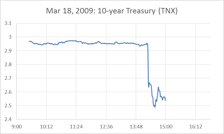
Movement of 10-year treasury on news of additional QE. Source James Hamilton at econbrowser.com.

My reaction was "that's a big, sudden shift ... wait, wha?!?"

The 10-year treasury is not impacted by QE as I rather decisively showed in the data here, so why should it drop on news of additional QE? Hamilton continues: "But over the next few days, the yield started climbing back up. By the end of April, the 10-year yield was higher than it had been before the Fed’s announcement." Hamilton then suggests and disproves that this was due to inflation expectations. The best answer seems to be that the market was wrong and then randomly drifted back to where it should be. [See diagram at the bottom of this post.]

[As an aside, market inflation expectations are also wrong.]

Note that I've discussed the idea that markets might not know what they are doing about a year ago to explain a set of observations from Scott Sumner about interest rates; the first two are here:

1. Moves toward easier money usually lower short term rates. The effect on long term rates is unpredictable.
2. Moves toward tighter money usually raise short term rates. The effect on long term rates is unpredictable.

The market appears to think monetary expansion lowers interest rates. However in the information transfer model (ITM) if inflation is high (the IT index 'kappa' is low), monetary expansion will lead to higher interest rates though the income/inflation effect. If inflation is low (kappa is high), then monetary expansion will lead to lower interest rates since the income/inflation effect is muted. I then explained Sumner's rules like this:

1. Markets like what they think is easier money, but the long run depends on whether the information transfer index is high or low. 
2. Markets don't like what they think is tighter money, but the long run depends on whether the information transfer index is high or low.

If the market knew how monetary expansion impacts interest rates, then we wouldn't get things like the incorrect adjustment in the graph at the top of this post.

Another potential area where the market appears to be in error is in exchange rates. The immediate response to expansionary policy in Japan and the Eurozone were a falling Yen and Euro ... but the Euro should rise if the supply of Euros expands because relative demand for currency explains the behavior of exchange rates, thus more Euros means more demand for Euros.

There are two takeaways from this:

• Since "the market" appears to have something like a monetarist view, immediate market responses to news should confirm e.g. Scott Sumner's model. The Fed announces QE, and the market expects a rise in the stock market, lower interest rates, a fall in the dollar and a return to target inflation. The market moves are taken as evidence that the Fed hasn't "run out of ammunition". However, in the long run, the economy moves back towards the ITM trends ... and you get pieces from Sumner like this: Were market monetarists wrong about Japan?
• If the market frequently moved in the wrong direction in particular venues, that would become a source of excess volatility. I'm not saying all venues! There are many where things where the market appears to get things right. However, there are excess volatility problems in exchange rates (mentioned above) and stocks [pdf].

Regarding the stocks, James Hamilton closes his post with a question about whether the rise in the Nikkei on news of QE from the BoJ will last. If stocks rise on what the market believes is good macro news, then if that belief is incorrect and the news should be considered neutral (e.g. QE) from the correct model, then there will be excess volatility and market moves should be discounted [1].

This also implies that market monetarism won't work. No matter the market expectations set by forward guidance or NGDP targets, they won't lead to the desired outcomes unless the underlying model is correct. You could guide inflation and NGDP with the ITM if it is correct -- but then if the ITM is correct, only certain values of NGDP growth and inflation are attainable.

Schematic drawing. Market belief in purple and the correct model in orange. The market considers neutral news to raise the given price, overshoots and returns to the original price.

[1] These are theoretical musings, and the ITM may well be wrong. Actually, the ITM does not as yet predict when the prices should return to trend (the market can be irrational far longer than you can remain solvent). So if you lose money shorting the Nikkei based on this low-traffic blog by a non-economist, it's your own fault.

Because empirical success

I've occasionally had discussions with some commenters, most recently Philippe on this thread, that such and such explanatory variable can't possibly be used to explain what I'm trying to explain because it doesn't make sense to that commenter. In the recent case, Philippe suggested that it didn't make sense that physical currency (the currency component of the monetary base, which I call M0) was an explanatory variable for inflation. Philippe suggested other forms of money that should matter for inflation, like M1 or central bank reserves.

You could probably put the brief back and forth between Nick Rowe and myself in the previous few posts into this framework, except in that case I'm disagreeing with Nick by saying expectations (the explanatory variable) can't explain the price level or inflation. Nick suggests that expectations (and central bank targets or guidance) are an explanatory variable, while I'm saying expectations do not explain much more than the most recent NGDP and M0 numbers.

Maybe the information transfer model is wrong and expectations and M1 matter for inflation. Whatever model you have, though, it can't be too different from the ITM. Why? Because empirical success. Here are the information transfer model results for the price level and inflation. First, here they are for the core PCE measure:

And here are the results for core CPI:

This is more empirically successful than any economic model of inflation that has ever been published. The P* model from the Federal Reserve was comparable in the 1990s, but choked on new data. Maybe the ITM will choke on new data, too. However, time and data will tell, not theoretical arguments. The details of the model are all written down in the "for beginners" posts linked on the sidebar of this blog. Have a go yourself! All of the data I've used is from FRED (except the Japanese monetary base data, which is from here).

Also note that the fact that both fits are good means that core PCE and core CPI inflation are not independent measures. The information transfer model describes them both equally well given the data we have, so there is no telling which is the "real" measure of inflation. What is interesting is that this observation follows regardless of whether you believe the information transfer model or not. The ITM fit to each measure implicitly defines a global transformation you can perform to turn CPI data into PCE data meaning that PCE = f(CPI) so that any property of CPI can be mapped to a property of PCE. The next time you see an economist chide someone for confusing the two measures, you can come to the rescue with the retort: there is no economically meaningful difference in PCE or CPI inflation. It's like the fact that there is no physically meaningful difference in measuring distances in kilometers or miles.

And it's not like the model for the US is a fluke; here is Japan:

The empirical accuracy doesn't mean various theoretical criticisms of the information transfer model are prima facie wrong; it just means they should be discounted (i.e. given a low prior probability of being correct) unless they are accompanied by a model of comparable empirical success. Or as I said to Philippe:

The benefit of using M0 as the explanatory variable for inflation is that it gives an incredibly accurate model. If you have done [sic] better model that uses M1 or MB that explains the price level, I'm interested in hearing about it! But if you're just making hand waving arguments without any empirical evidence, that seems like a step backwards from the ITM.

The ITM doesn't just do inflation -- the interest rate model is pretty good too:

If you're of the opinion that the Fed's expansion of reserves will result in inflation, that people's expectations matter, or even that human decisions and behavior matter in a macroeconomic system at all, I'd first like to see some lines going through some data points.

Update 7:30pm MST, for Nick's comment below: 

Both of the error results for the PCE and CPI inflation models above have approximately zero mean. First, PCE inflation error:

Second, CPI inflation error:

In which I irritate Nick Rowe (again)

I am currently on travel for work (again) so light updates this week, but I thought I could irritate Nick Rowe some more. He has a new post up where he shows how police could regulate the speed of drivers without actually pulling anyone over:

http://worthwhile.typepad.com/worthwhile_canadian_initi/2014/11/the-collective-speed-limit-game.html

I took on two other analogies before here:

http://informationtransfereconomics.blogspot.com/2014/10/the-trouble-with-nick-rowes.html

... and my critique is similar this time.

The speed limit analogy would make sense if we all had NGDP/inflation meters/pedals. However, since many of the influences that go into NGDP or inflation are beyond our control, it's hard for individuals to target them.

A restaurant owner can't have her patrons enjoy the food 1% more while paying 3% more (to hit 2% inflation, including quality adjustments). She can't help it if suddenly her chief ingredients become cheaper and competition forces her to reduce prices ... This has been happening in the computer industry for awhile now, with actual deflation in the tech sector price level.

That's the gist of the linked post; here's some new stuff.

1.

A tiny tweak to the behavior model turns the speed limit equilibrium into a boom-bust cycle. If the police don't pull anyone over (and no one is being seen being pulled over), people will start to speed more often and the police will start having to pull people over (concrete steps). Eventually enough people are pulled over (or witness such events) that leads back to the zero-enforcement scenario. Which leads to speeding and the cycle begins anew.

In the economic version, you'd see central bank targets start to lose their effectiveness, followed by concrete steps.

2.

You can get the same speed limit equilibrium without expectations. In an ideal gas the velocity of particles follows a maxwell Boltzmann distribution with average speed ~ kT. Nothing actually acts on the molecules to achieve this at the micro level -- the effect of the cops in this case is an emergent entropic force that does not exist for individuals.

3.

If Inflation and demand don't actually exist at the micro level, then the speed limit analogy doesn't make any sense at all. We can't measure our individual speed much like an individual molecule doesn't have a temperature. There is nothing to expect! You can't get tickets for going "undefined" ...

[This is not a very good post. BTW I'm writing it in a hotel room down the street from the St Louis Fed with one finger on my iPad, hence the picture above.]

The information transfer model and the econoblogosphere

Paul Krugman has a post up that criticizes the "neo-Fisherite" view. Oddly I completely agree with his post, yet I wrote a post about agreeing with John Cochrane's post, which Krugman calls the "highest level" of  Keynesian denial. It might be confusing as to exactly where I or the information transfer model (ITM) stands.

I wrote two posts in the past that illustrate a bit of how the ITM fits in with both the history of macroeconomic thought and the debate around the current crisis. Actually, the ITM can help explain the history of macroeconomic thought. At its heart, the ITM says Paul Krugman is always right, but not necessarily for the right reasons. Anyway, this is a post fleshing that statement out with a bit more detail in fun, easy to read listicle format.

First, let me say that the ITM has a critical parameter κ (kappa, basically named after the parameter in this paper by Fielitz and Borchardt), called the information transfer index. In short, it represents the relative size of information chunks received by the supply and transmitted by the demand. Anything you say about the information transfer model has a caveat depending on the value of κ. There are two major κ regimes, and they're not very far apart numerically. When κ ~ 0.5, the ITM reduces to the quantity theory of money (and is similar to the AD/AS model with monetary offset). When κ is larger, getting towards κ ~ 0.8 to 1.0, the quantity theory stops being a good approximation to the ITM and the IS-LM model becomes a better approximation. The details are linked at this post. 

The thing is that κ can change over time and is different for different countries. That ends up muddling things a bit so I end up agreeing with Scott Sumner, Nick Rowe, Paul Krugman, David Glasner, or John Cochrane on various occasions and disagreeing with them on other occasions.

One additional detail is that the ITM says that κ tends to rise as economies get bigger and can only be reset by changing the definition of money or a monetary policy regime change. Hence you can consider old/advanced economies as generally having larger κ while younger emerging economies have lower κ. This is not always true, but can be a good guide. With that bit of background, on with the listicle!

Expectations

I personally think the way expectations are used in macroeconomics make the field unscientific. They appear to be important in microeconomics (and game theory) -- and I have no particular problem with the way they are used there. However, mainstream macroeconomics does not appear to have any kind of constraints on what form expectations take, and hence allow anything to happen in a model. This reaches an almost absurd level with e.g. Nick Rowe's insistence that if a central bank is credible with its NGDP (or inflation) target, the economy will reach that NGDP (or inflation) target ... without the central bank actually having to do anything (besides 'be credible'). I've encountered many other theories and papers in my short few years of studying economics that effectively assume the conclusion through expectations. One economist called these chameleon models (although the author does not specifically call out expectations as the source ... however the questionable assumptions in economic models are typically about expectations or human behavior).

That aside, in the information transfer model, 'expectations' as such take the specific form of probability distributions over market variables (they parameterize our ignorance of the future). Since these distributions always differ from the actual probability distributions (we do not have perfect foresight), they represent information loss and hence a drag on economic growth (relative to perfect foresight). Additionally, prices are not only lower than they would be if we knew the actual probability distribution of market variables, but frequently lower than if we parameterized our ignorance as maximal (which is what the information transfer model does).

The monetary base

The monetary base is directly related to short term interest rates in the ITM. However, only the currency component of the monetary base (I've called it M0 as they have in the UK in the past) has any impact on inflation and then only when κ is closer to 0.5. Monetary base reserves have little to do with inflation ... except in the sense that movements in reserves can sometimes cause movements in the currency base.

Liquidity trap

The ITM model has a lot of similarities with the liquidity trap when κ ~ 1.0 -- I've called it the "information trap". Monetary policy does not have strong impact -- neither raising nor lowering interest rates, nor expanding nor contracting the currency base. The "information trap" differs from the modern liquidity trap in that it doesn't have to happen at the zero lower bound (ZLB) ... it is more like Hawtrey's credit deadlock or Keynes original liquidity trap that didn't have to happen at the ZLB. 

The ITM is, in a sense, identical to Paul Krugman's mental model (or what seems to be his mental model) if you replace "normal times" with κ ~ 0.5 and "liquidity trap" with κ ~ 1.0.

The Phillips curve

This sounds reasonable, but doesn't appear to have a strong signal in the data using the ITM. The two variables (inflation and unemployment) have a complicated relationship and the ITM doesn't describe the fluctuations leading to unemployment -- unemployment seems to be the result of, for lack of a better set of words, irrational panic that could only be modeled by modeling human behavior.

(New) Keynesianism

Essentially, the ITM is well-approximated by the ISLM model when κ ~ 1.0, but not when κ ~ 0.5. So the ITM is sometimes Keynesian inasmuch as the ISLM model is Keynesian. New Keynesianism is based on the expectations-augmented Phillips curve. Given what I've said about expectations and the Phillips curve above, you can guess that the ITM probably doesn't agree with new Keynesian methodology. This isn't to say the models are wrong or won't outperform the ITM against data -- just that methodologically they represent completely different viewpoints. 

Also, since in the US κ has been close to 1.0 both today and during the 1920s-30s, the ITM basically says Keynesianism has been the right theory at those times ... as Paul Krugman says, our world today (and Japan in the 90s) represents the return of depression economics.

(Market) Monetarism

If you take out the expectations piece (the "market" in market monetarism) ... and instead of M2 or MB use M0 ... and give a specific form for the velocity of money, the ITM basically agrees with monetarism ... when κ ~ 0.5. That is to say that Milton Friedman was (almost) right about the US during the 1960s and 70s (but wrong about Japan and the Great Depression). Scott Sumner and Nick Rowe are also right about the 1970s. Additionally, κ < 1.0 for Canada, Australia, China, Russia and Sweden (currently), so monetarism gets those right. However monetarists frequently try to appeal to data from these countries to prove their point about the US, Japan or the EU; in the ITM this is comparing apples and oranges.

Neo-Fisherite model

The only two things that the ITM has in common with this idea/model is that lower interest rates run you into low inflation faster than higher interest rates, and, if κ gets too large, the dependence of the price level on M0 (currency base) becomes an inverse relationship ... i.e. deflationary monetary expansion (as evidenced by Japan). This latter mechanism will lead to even lower interest rates over time.

However! An economy with a constant rate of inflation and a constant interest rate is impossible (unless RGDP grows at an increasingly exponential rate), and the mechanism has nothing to do with expectations, but rather is closely related to the liquidity trap. This makes it different from the typical neo-Fisherite view.

Fiscal policy

Debt-financed fiscal policy always boosts NGDP as it represents an independent process from economic growth. It also raises interest rates (aka 'crowding out'). However, when κ ~ 0.5, if the central bank is targeting inflation or NGDP, fiscal policy will fail to produce inflation (or NGDP) due to monetary offset (q.v. Scott Sumner). When κ ~ 1.0, then there is no monetary offset and the impact on interest rates is minimal. Again this view almost perfectly matches up with Paul Krugman's views, except that "liquidity trap conditions" mean κ ~ 1.0.

(My personal politics on this issue say that even if e.g. unemployment insurance negatively impacted NGDP, we should still do it because we are human beings not heartless automatons optimizing economic variables.)

Coordination failures

David Glasner and Nick Rowe have several posts that present the idea that coordination failures are the cause of recessions (Nick Rowe tends to put the onus on monetary policy, while David Glasner does not). The ITM motivates the idea that coordination causes the recession in the first place (i.e. people en masse becoming pessimistic about the economy) and that the economy does not naturally re-coordinate (create the 'inverse coordination' of the original pessimism) in order to undo that loss in NGDP. That re-coordination would require resources (e.g. debt financed fiscal policy) comparable to the original NGDP loss ... basically the idea that government spending should approximately equal the output gap per Keynesian analysis.

Other ideas?

...