Equilibria

This is a somewhat rambling post about equilibria; it has been sitting around for a few days. I thought I'd publish it even though I'm still thinking about the issues at hand.

Anyway ... there has been a diffuse thread about nonlinear models and multiple equilibria in the econoblogosphere over the past few weeks. I was mostly confused about Farmer's comments on a post of David Glasner's (summarized here) where he said there was a continuum of equilibria:

Farmer:

I like Lucas’ insistence on equilibrium at every point in time as long as we recognize two facts. 1. There is a continuum of equilibria, both dynamic and steady state and 2. Almost all of them are Pareto suboptimal.

Glasner responded in part:

I think equilibrium at every point in time is ok if we distinguish between temporary and full equilibrium

Farmer later says:

A linear model can have a unique indeterminate steady state associated with an infinite dimensional continuum of locally stable rational expectations equilibria. A linear model can also have a continuum of attracting points, each of which is an equilibrium.

We must realize here that Farmer is throwing away Arrow-Debreu. The Hopf index theorem shows that the Arrow-Debreu equilibria (in the case where there isn't a unique equilibrium) are locally unique (isolated zeros of the excess demands vector field).

I asked Farmer on his blog about that ... and he says indeed he is:

Yes. I'm abandoning Arrow Debreu and replacing it with competitive search [pdf] (with a Keynesian twist).

I did consider that maybe it was possible to interpret this as Arrow-Debreu isolated zeros (zero excess demand vectors) in the n-dimensional price vector space that are part of a dynamic continuum in the time dimension -- even going so far as to draw this diagram in my notes:

At first I thought that those temporal paths (red) couldn't cross each other as it would violate the Hopf theorem (non-isolated zeros) ... however, the zeros can have multiplicity -- it would be much like how the quadratic equation (x - 2)^2 has two solutions at x = 2. That crossing path would be modeled something like the solution to this quadratic equation:

(x - 2 - ɛ) (x - 2 + ɛ) = 0

with ɛ → 0. However, neither the crossing of the paths nor the Arrow-Debreu equilibria are important given Farmer's response.

Overall, I was confused more by this. It seems Farmer is saying most every state we observe the economy in is an "equilibrium" ... that it is a solution to a set of equations. And now I think Noah Smith might (snarkily) have been subconsciously subtweeting Farmer when he wrote:

Economists have re-defined "equilibrium" to mean "the solution of a system of equations". Those criticizing econ should realize this fact.

Brad DeLong responded Noah Smith with essentially my sentiment towards Farmer's new definition of equilibrium ...

@noahpinion (1/2) why not use “solution to a system of equations” to mean “solution to a system of equations”, and reserve “equilibrium” 

(2/2) for “the matching of transactors to transactions” leaves few and roughly balanced unsatisfied buyers and sellers?

Hear, hear! Krugman had some commentary on Farmer as well ...

In part, I think, Farmer is trying to explain an empirical regularity he thinks he sees, but nobody else does — a complete absence of any tendency of the unemployment rate to come down when it’s historically high. I’m with John Cochrane here: you must be kidding.

I think you can make this even stronger (and snarkier) as I do here:

Another (snarky) way to put it is that a naive ... [ADM] equilibrium employment rate [note: not unemployment] is predicted to be 100%. The current value? 93.7%. Here is a graph of the naive equilibrium model and the slightly improved natural rate model:

 

Economists don't tend trot this plot out (maybe they should?) because they're more interested in the deviations from equilibrium. It's actually rather amazing that the [ADM equilibrium] model should work this well!

But then I also speculated that one could see multiple equilibria in the unemployment data:

However most of the equilibria are near the "natural rate" defined by the information transfer model P : N → U and the metastable red and green patches are more of an epi-phenomenon. In fact, there was no pause in the fall in the unemployment rate just below 8% in the recent recovery (there was no red patch in mid-2012), so maybe these states aren't real at all.

Basically, I see information equilibria as the proper equilibria -- maximum entropy configurations of two macroeconomic aggregates in information equilibrium with each other. In the labor market we have P : N → U, i.e. P ~ N/U (or log N ~ k log U) is an equilibrium condition. But that is only approximate and there is a slight drift towards higher unemployment rates:

I think this drift (unit root) is not real, though ... in fact, I think it is a missing piece of the model that I don't have a good explanation for but affects both markets P : N → U and P : N → L (L is the total employed). That is to say we are seeing either more output or fewer people employed than we expect as time passes.

Is this the long lost total factor productivity? Is it just capital in the Solow production function?

At this point I am just rambling on. See the note at the top of this post ...




Update (+1 hr): It seems David Glasner had some of the same questions I had -- and more interesting different ones:

http://uneasymoney.com/2015/04/29/roger-and-me/

The new NGDP numbers are here ...

And the new GDP data is out! A pretty dismal performance ... but then the Atlanta Fed was saying Q1 seems to come in low these days (H/T to Cullen Roche who also had a good prediction), and in fact pretty much nailed the number with their GDPNow forecast.

I marked the Q1 numbers with blue dots on the prediction graph -- they do seem to have been systematically low since the financial crisis.

Overall: a continuing a trend of lukewarm economic performance, largely still in line with just about any model of the economy.

Economic potentials or: How to define an economy

I'm attempting to construct the thermodynamic potential for an economy by elaborate analogy -- demand/output is analogous to energy, price to pressure and supply to volume. What does this help with? For one thing, it leads toward a way to introduce a chemical potential (which after writing this post, I realize might not be necessary). However, it also allows for a way to organize thought around microeconomic and macroeconomic forces (see e.g. here or here).

Using the definitions here and here (and writing $N$ for nominal output, $X$ for goods with price $p$ -- which could be taken to be  the price level $P$ but we'll leave separate for now, $T$ for the 'economic temperature' and $S$ for the 'economic entropy' -- the latter two being defined at the links), we have for a monetary economy:

$$
N = TS + \kappa P M + \alpha p X
$$

$$
N \approx c N/\kappa + \kappa P M + \alpha p X
$$

where we use Stirling's approximation (with large $N$, but small changes) and the definitions

$$
S \sim \log N! \approx N \log N - N  \;\;\text{ and }\;\; 1/T \sim \log M
$$

with $M$ being the money supply (empirically, base money minus reserves) and $\kappa = \kappa (N, M)$ being the information transfer index for the money market. Note that $\kappa \sim 1/T$ so that high $\kappa$ represents a low temperature economy and vice versa.

For multiple goods we have [1]

$$
N =  T S + \kappa P M + \sum_{i} \alpha_{i} p_{i} X_{i}
$$

where the sum is over the individual market "generalized forces" (microeconomic forces). For example, we can look at a simple model of an aggregate goods market $A$ and a labor market $L$:

$$
N =  T S + \kappa P M + \alpha P A +  \beta P L
$$

... all prices for labor and goods are taken to be proportional to the price level. This allows us to organize microeconomic and macroeconomic forces

$$
N =  \underbrace{T S + \kappa P M}_{\text{macro forces}} + \underbrace{\alpha P A +  \beta P L}_{\text{micro forces}}
$$

In truth, the $P M$ component should probably be considered a microeconomic force (since it behaves like one for the most part) and only $TS$ -- the entropic forces -- should be considered macroeconomic forces. However, since $P M$ is a large component of the economy (and would likely be for a commodity money system as well, see footnote [1]) and policy-relevant, I'll keep it in. Understanding this distinction would point towards (using the separation from this earlier post about a financial and government sectors $F$ and $G$):

$$
\text{(1) } N =  T S + \kappa P M + \alpha P A +  \beta P L + \gamma P G + \epsilon i F
$$

where $i$ is a general market index (e.g. the S&P500 could be used). This approach can be compared with the older approaches that use the definition of nominal output:

$$
N = C + I + G + NX
$$

where we'd instead write (for example, assuming the prices are all proportional to the price level $P$):

$$
\text{(2) }N = a_{1} P C + a_{2} P I + a_{3} P G + a_{4} P NX
$$

The $a_{i}$ are all constants. Comparing equations (1) and (2) we can see that they mostly just represent different partitions of nominal output. Equation (2) lacks an explicit monetary component, but the biggest difference is that it lacks an 'entropic' component $T S$. I'd visualize $T S$ as the additional gains in welfare from exchange -- exchange makes both parties better off and increases the value of whatever it is that is exchanged.

Another topic that becomes clearer with the construction (1) is that of monetary vs Keynesian takes on macroeconomic stabilization. In (1), it becomes clear that a change in $G$ could be offset by a change in the $\kappa P M$ term or even the $T S$ term in general. In practice it depends on the details of the model (specifically the value of $\kappa$ -- if it is near 1 changes in $M$ have limited impact, and if it is near 1/2 you have an almost ideal quantity theory of money).

Additionally, the conditions that allow monetary offset of fiscal stimulus to occur also allow the monetary offset of the effects of a financial crisis. At least if (1) is a valid way to build an economy.

This last piece is interesting -- it implies that financial crises cause bigger problems in a liquidity trap economy ($\kappa \sim 1$). Assuming the model is correct, the reason the global financial crisis was so bad was because it struck when $\kappa \sim 1$ for a large portion of the world economy: the EU, US, and Japan. Other financial crises (e.g. 1987 in the US or even the dot-com boom) struck at a time when $\kappa < 1$ and were better able to be offset by monetary policy.

Footnotes:

[1] Actually, the $\kappa P M$ component is like one of the goods markets and in e.g. a commodity money economy, it would be one (and entropy should be defined in terms of that good). However it may be more useful to separate it as a macroeconomic force as is done later in the post.

Happy birthday to this blog

This blog is now 2 years old and is heading towards 500 posts. I thought I'd celebrate with a countdown listicle of some of the least viewed posts here.

At 28 pageviews we have ...

What does E_t π_t+1 mean?
This post was actually pretty weird (with a weird graphic) -- mostly me thinking out loud about the possible meaning and consequences of expectations terms in DSGE-type models as they essentially couple the future to the past.

At 25 pageviews we have ...

Do the different market models work simultaneously?
This was a response to LAL who has become a frequent commenter since that time about whether the models of the labor market, interest rates, capital, etc worked simultaneously. It has a cool diagram.

At 17 pageviews we have ...

Powerful evidence for the information transfer model
The data appear to rather unambiguously support the model log N ~ k log M with k falling.

And finally in last place with 10 pageviews we have ...

Below target inflation
This is a paper that can be interpreted as confirming the slowing of inflation over time.

...

The key takeaway seems to be that Monday evening is a bad time for posting ... so happy Friday morning everyone.

How not to apply math and physics to economics

I started following the Real World Economics Review (RWER) blog -- a capital-H Heterodox outlet -- in order to branch out and see if anyone might be interested in my information theory take. I continue to follow it because it is a source of great entertainment. Take Asad Zaman:

This essay [on Godel's Theorem] shows that logic is limited in its ability to arrive at a definite conclusion even in the heartland of mathematics. Pluralism is required to cater for the possibility that both Euclidean and non-Euclidean geometries represent valid ways of looking at the world. The world of human affairs is far more complex. In order to study and understand societies, one must learn to deal with a multiplicity of truths. ... These ideas form part of the background for supporting the drive for pluralism in our approaches to economic problems.

Godel's theorem applied to axiomatic systems of comparable power to the Peano axioms and proves the existence of theorems about natural numbers that cannot be proven true or false given the axioms.

Things not proven by Godel:

• Physically relevant models (to a given level of approximation) of the universe (economics included) are among those theorems
• You cannot empirically validate a 'theorem' about a physical (or economic) system
• There exists other forms of reasoning that can reach these true or false but unprovable theorems

Actually, what's funny is that what Godel essentially proves is that there exists a statement in mathematics that is roughly equivalent to "This sentence is false." in English. The existence fo that statement in English (and most if not all other languages) would then mean, by Zaman's logic, that language is limited in its ability to solve economic problems. Interpretive dance comes to mind. But it may be possible to construct a dance move that is its own negation ...

Then there is that nonsense about geometry. Euclidean and non-Euclidean geometries are not different ways of looking at the world; they are subsets of one way of looking at the world called "geometry". They actually both exist simultaneously in General Relativity -- space is both flat (Euclidean geometry) and curved near massive objects (non-Euclidean geometry). Another way to put it: Euclidean geometry is an approximation to non-Euclidean geometry for small values of curvature.

Also, the parallel postulate is not an "unprovable" statement in the Godel sense, it is actually just something that is true in Euclidean geometry -- i.e. not true in the general case.

In fact, the "unprovable" statements out there that could be taken as examples of Godel's undecidable propositions are very abstract ... like the continuum hypothesis or the axiom of choice. As I was never one for formal logic (my math degree concentrated on group theory and topology), I'm not sure these really count as undecidable propositions in the Godel sense. Wikipedia says they do, but I'm not inclined to believe that. Both of these are independent of the Peano axioms -- a bit like saying "my hair is brown" is independent of the Peano axioms.

I also learned of Nicolas Georgescu-Roegen and his book "The Entropy Law and the Economic Process" from RWER. I was intrigued, but soon learned that Georgescu-Roegen posited the idea of the "arithmomorphic fallacy", which is not a fallacy but in fact an assertion of the sort that I tend to file under the "failure of imagination fallacy". Just because you can't think of the way of describing something with mathematics doesn't mean there isn't a way. That is a genuine fallacy. It is even entirely plausible that our entire universe is the product of computations with the bits on a holographic screen at the cosmological horizon -- and is therefore entirely made of math.

Georgescu-Roegen did have an interesting contribution to ecological economics in recognizing the fact of  a finite entropy production between the current state of the solar system and its eventual "heat death". Besides free energy (or enthalpy) being the more relevant functions, the scale of entropy production is so immense (the largest contributions are from sunlight warming the planet and the water and carbon cycles) that the human impact -- stemming almost entirely from global warming (impacting the carbon cycle) -- amounts to only a tiny fraction. From the perspective of the empirical values of entropy production, global warming would be the only ecological problem you would worry about. 

This is not a reason to not care about the environment ... it's just a unnecessarily general and abstract reason. Graham's number comes to mind (possibly the worst upper bound for a result ever constructed). It would probably be better to say that the surface area of the Earth is finite, therefore let's not cover it all with trash and cities.

NGDP prediction updates

Nine days until the BEA releases its first estimate of Q1 NGDP. I've been updating the prediction graph with the predictions from hypermind linked at Scott Sumner's blog (see here, here) -- the Q1 prediction has been falling towards the advance estimates. And the advance estimates appear to be low ... in the area of 1.2% growth (see e.g. here).

The information equilibrium model doesn't get so detailed ... all of these estimates are within the error probability. Here's the original prediction. And here's the updated graph:

Here are the historical Hypermind predictions for Q1 NGDP growth:

You can clearly see the "update" that happens as 2014Q4 data is released at the end of January, as well as smaller "updates" around CPI inflation data releases at the beginning of each month.

Do macro models need a financial sector?

Dan Davies had this analogy on twitter for macro without a financial sector:

@dsquareddigest: @Frances_Coppola @ericlonners it's as if there was an epidemic of hepatitis and half the doctors had to look up what the liver was for.

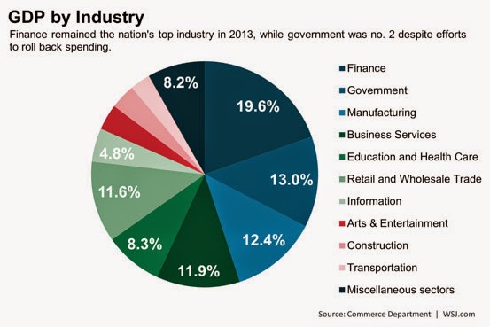
And if we look at e.g. the data presented in this blog post, we can see that the financial sector is indeed a sizable chunk of NGDP at 19.6% in 2013.

Let's try to build a picture of what such a "financialized" economy looks like starting from the maximum entropy view of the information equilibrium model. Borrowing pictures from that post, a snapshot of an ordinary economy looks something like this:

Each box represents a business or industry, and at any time they might find themselves on the decline or growing, with most growing near the average rate of economic growth for the whole economy.

As we can see in the pie chart, though, there should be at least one very large box that moves in concert: the government. Generally, due to coordination by the legislative branch, government spending can move as a single unit -- e.g. across the board spending or tax cuts.

Now inside a single industry, the individual units won't necessarily be coordinated -- in fact, e.g. Ford and GM might be anti-correlated with one surging in profits while the other loses market share. Domestic manufacturing in general can rise or decline (crowded out by imports), but overall the result will be a lot less coordinated than government spending (except e.g. in a recession when all growth slows).

But what if the other big slice in the pie chart is coordinated? The financial sector could be as coordinated as government spending with markets effectively acting as the legislative branch. If we put government and the financial sector (to scale) in our snapshot, we get something that looks like this:

I've put government (in blue) growing at roughly the modal rate and the financial sector (in gray) outperforming it.

Now I've already looked at what happens when the government sector moves around; what we're concerned with today is the financial sector. If the financial sector is coordinated (through market exchanges or inter-dependencies), a big financial crisis can make the entire sector enter a low growth (or declining) state like this:

This is a far more serious loss of entropy than an uncoordinated sector of the same size with 50% (coordinated fraction = 0.5) of the states going from growth states to declining states, pictured here:

A calculation using the Kullback-Liebler divergence has the former version resulting in a loss of entropy of 4%, while the latter loses only 1%. In general, it looks like this:

One way to visualize the uncoordinated case is the dot-com bust where there were many different actors in the sector as opposed to the relatively smaller number of  financial companies (q.v. "contagion") in the highly coordinated case.

Simply because it represents a large fraction of the US economy and is highly coordinated by exchanges (a significant bad day on the S&P500 is usually a significant bad day on other exchanges -- even around the world), it is plausible to posit the financial sector can move as a single unit, much like the government sector (coordinated instead by political parties).

We can think of the financial sector F as analogous of a second "government" sector and write:

NGDP = C + I + F + G + NX

(This is a heuristic designation -- F would specifically be carved out of C, I, G and NX as appropriate, and the exact definition would take some econometrics work.)

Financial crises would be much like government austerity, except they would be by definition procyclical -- being more likely when a recession happens, being the cause of a recession [1], or even being synonymous with a recession. A surging market is not very different from a surge in government spending; a collapsing market is not very different from a fall in government spending. That is to say a good model of the financial sector would simply be to dust off those old models of the government sector.

Footnotes:

[1] I still think of recessions as avalanche events, but the financial sector can be the large rock that precipitates the cascade.

Diamond-Dybvig as a maximum entropy model

I'm pretty sure this is not the standard way to present Diamond-Dybvig (which seems more commonly to be presented as a game theory problem).  However, this presentation will allow me to leverage some of the machinery of this post on utility and information equilibrium. I'm also hoping I haven't completely misunderstood the model.

Diamond-Dybvig is originally a model of consumption in 3 time periods, but we will take that to be a large number of time periods (for reasons that will be clear later). Time $t$ will be between 0 and 1.

Let's define a utility function $U(c_{1}, c_{2}, ...)$ to be the information source in the markets

$$
MU_{c_{i}} : U \rightarrow c_{i}
$$

for $i = 1 ... n$ where $MU_{c_{i}}$ is the marginal utility (a detector) for the consumption $c_{i}$ in the $i^{th}$ period (information destination). We can immediately write down the main information transfer model equation:

$$
MU_{c_{i}} = \frac{\partial U}{\partial c_{i}} = k_{i} \; \frac{U}{c_{i}}
$$

Solving the differential equations, our utility function $U(c_{1}, c_{2}, ...)$ is

$$
U(c_{1}, c_{2}, ...) = a \prod_{i} \left( \frac{c_{i}}{C_{i}} \right)^{k_{i}}
$$

Where the $C_{i}$ and $a$ are constants. The basic timeline we will consider is here:

Periods $i$ and $k$ are some "early" time periods near $t = 0$ with consumption $c_{i}$ and $c_{k}$ while period $j$ is a "late" time period near $t = 1$ with consumption $c_{j}$. We introduce a "budget constraint" that basically says if you take your money out of a bank early, you don't get any interest. This is roughly the same as in the normal model except now period 1 is the early period $i$ and period 2 is the late period $j$. We define $t$ to be $t_{j} - t_{i}$ with $t_{j} \approx 1$ so the bank's budget constraint is

$$
\text{(1) }\;\; t c_{i} + \frac{(1-t) c_{j}}{1+r} = 1
$$

The total available state space is therefore an $n$-dimensional polytope with vertices along axes $c_{1}$, $c_{2}$, ... $c_{n}$. For example, in three dimensions (periods) we have something that looks like this:

Visualizing this in higher dimensions is harder. Each point inside this region is taken to be equally likely (equipartition or maximum information entropy). Since we are looking at a higher dimensional space, we can take advantage of the fact that nearly all of the points are near the surface ... here, for example is the probability density of the location of the points in a 50-dimensional polytope (where 1 indicates saturation of the budget constraint):

Therefore the most likely point will be just inside the center of that surface (e.g. the center of the triangle in the 3D model above). If we just look at our two important dimensions -- an early and late period -- we have the following picture:

The green line is Eq. (1) the bank's budget constraint (all green shaded points are equally likely, and the intercepts are given by the constraint equation above) and the blue dashed line is the maximum density of states just inside the surface defined by the budget constraint. The blue 45 degree line is the case where consumption is perfectly smoothed over every period -- which is assumed to be the desired social optimum [0]. The most likely state with equal consumption in every period is given by E in the diagram.

The "no bank" solution is labeled NB where consumption in the early period is $c_{i} \approx 1$. The maximum entropy solution where all consumption smoothing (and even consumption "roughening") states are possible because of the existence of banks is labeled B.

The utility level curves are derived from the Cobb-Douglas utility function at the top of this post. You can see that in this case we have B at higher utility than E or NB and that having banks allows us to reach closer to E than NB.

If people move their consumption forward in time (looking at time $t_{k} < t_{i}$), you can get a bank run as the solution utility (red, below) passes beyond the utility curve that goes through the NB solution. Here are the two cases where there isn't a run (labeled NR) and there is a run (labeled R):

Of course, the utility curves are unnecessary for the information equilibrium/maximum entropy model and we can get essentially the same results without referencing them [1], except that in the maximum entropy case we can only say a run happens when R reaches $c_{i} \approx 1$ (the condition dividing the two solutions becomes the consumption in the early period is equal to the consumption in the case of no banks, rather than the utility of the consumption in the first period is equal to the utility of the consumption in the case of no banks).

I got into looking at Diamond Dybvig earlier today because of this post by Frances Coppola, who wanted to add in a bunch of dynamics of money and lending with a central bank. The thing is that the maximum entropy approach is agnostic about how consumption is mediated or the source of the interest rate. So it is actually a pretty general mechanism that should be valid across a wide array of models. In fact, we see here that the Diamond Dybvig mechanism derives mostly from the idea of the bank budget constraint (see footnote [1], too), so in any model where banks have a budget constraint of the form Eq. (1) above, you can achieve bank runs. Therefore deposit insurance generally works by alleviating the budget constraint. No amount of bells and whistles can help you understand this basic message better.

It would be easy to add this model of the interest rate so that we take (allowing the possibility of non-ideal information transfer)

$$
r \leq \left( \frac{1}{k_{p}} \; \frac{NGDP}{MB} \right)^{1/k_{r}}
$$

This would be equality in the ideal information transfer (information equilibrium) case. Adding in the price level model, we'd have two regimes: high and low inflation. In the high inflation scenario, monetary expansion raises interest rates (and contraction lowers them); in the low inflation scenario, monetary expansion lowers interest rates (and contraction raises them). See e.g. here. I'll try to work through the consequences of that in a later post ... it mostly moves the bank budget constraint Eq. (1).

Footnotes:

[0] Why? I'm not sure. It makes more sense to me that people would want to spend more when they take in more ... I guess it is just one of those times in economics where this applies: ¯\_(ツ)_/¯

[1] In that case the diagrams are much less cluttered and look like this:

Micro stickiness versus macro stickiness

The hot topic in the econoblogosphere appears to be nominal rigidity. Here's Scott Sumner. Here's David Glasner. Here's my take on Glasner. Here are some other bits from me.

Anyway, I think it would be worthwhile to discuss what is meant by "sticky wages".

One way to see sticky wages is as individual wages that don't change: total microeconomic stickiness. This position is approximately represented by a paper from the SF Fed Sumner discusses at the link above. However the model they present not only doesn't look like the data at all, but is better representative of completely sticky wages than just sticky downward wages. It's so bad, I actually made a mistake looking at the model -- I didn't read the axes correctly as the central spike is plotted against the right axis. Here is a cartoon of what that graph should look like if the spike and the rest of the distribution were plotted on the same axes:

The light gray bars represents the distribution of wage changes at a time before the recession, the dark bars represent the same thing after a recession. Basically a big spike at zero wage change in both cases.

Another way to see sticky wages is as being sticky downward. This is how I originally looked at the model from the SF Fed. The picture you have is very few wage decreases -- mostly wage increases and zero changes -- and it represents individual sticky-downward wages (at the micro level):

These are the two sticky microeconomic cases.

Now what would sticky macroeconomic wages look like? There are two possibilities here: 1) wages are individually sticky and 2) wages are collectively sticky, but individually flexible. Case 1 looks like the SF model above -- a spike at zero -- or the downward rigidity in the second graph. 

Case 2 looks like a distribution with constant mean -- total nominal wages keep the same average growth before and after the recession. Individual wage changes fluctuate around from positive to negative. Case 2 is a bit harder to visualize with a single graph, so here is an animation:

The mean I am showing is the mean of the flexible individual wages, not the ones dumped into the zero wage change bin at the onset of the recession (I also exaggerated the change in the normalization at the onset of the recession so it is more obvious what is happening).

Here is what that case looks like in the same style as the previous graphs:

You may be curious as to why, even with the spike at zero wage change, I still consider wages to be "flexible" individually. In the case of the SF model, ~ 60-90% of wages are in the zero change bin; that's sticky. In all of the others, only ~10% of wages are in the zero change bin -- ~90% of wages are changing by amounts up to 20% or more. I wouldn't call that individually sticky at all. Additionally, before and after a recession, the fraction in the zero bin only goes up by a few percentage points.

And that is really what is happening! Here is the data from the SF Fed paper:

That looks like sticky macro, flexible micro wages (no change in the mean, individual changes of up to 20%).

Note also that this data looks nothing like the model presented in the paper (the first graph from the top above) or sticky downward individual wages (second graph from the top above).

There remains the question of whether there is any macro wage flexibility -- let's look at the case of flexible macro, flexible micro wages, again best seen as an animation. In this case the mean of the flexible piece of the distribution goes up and down:

How does this look if there's a recession and wage growth slows in the style of the graphs above?

This actually qualitatively looks a bit more like the data than the sticky macro, flexible micro case -- there are some light gray bars sticking out above the distribution on the right side as they do in the data. However that effect is pretty small; to a good approximation we have sticky macro, flexible micro wages.

The animation of the flexible macro, flexible micro case illustrates the theoretical problem brought up in Glasner's post:

This doesn’t mean that an economy out of equilibrium has no stabilizing tendencies; it does mean that those stabilizing tendencies are not very well understood, and we have almost no formal theory with which to describe how such an adjustment process leading from disequilibrium to equilibrium actually works. We just assume that such a process exists.

In a sense, he is saying we have no idea how the wages collectively move to restore equilibrium through individual changes. Nothing is guiding the changing location of the mean in the animation -- there is no Walrasian auctioneer steering the economy.

The sticky macro, flexible micro case solves this problem -- but only if the equilibrium price vector is an entropy maximizing state and not e.g. a utility maximizing state (see here for a comparison). Since the distribution doesn't change, there is no change requiring coordination of a Walrasian auctioneer. The process of returning to an equilibrium from disequilibrium is simply the process of going from an unlikely state to a more likely state.

Let me use an analogy from physics. Consider a box of gas molecules, initially in equilibrium at constant density across the box (figure on the left). If we give the box a jolt, you can set up a density oscillation such that more molecules (higher pressure) are on one side than the other (figure on the right):

Eventually the molecules return to the equilibrium (maximum entropy) state on the right left guided only by the macro properties (temperature, volume, number of molecules). The velocity distribution doesn't change very much (i.e. the temperature doesn't change very much). We simply lose the information imparted by the shock as entropy increases.

The disequilibrium state with higher pressure on one side of the box is analogous to the disequilibrium price vector described by Glasner. The macro properties are NGDP and its growth rate. The velocity distribution is analogous to the wage change distribution. And the process of entropy increasing to its maximum is the process of tâtonnement.

The key idea to remember here is that there is nothing that violates the microscopic laws of physics in the box on the right -- that state can be achieved by chance alone! It's just very very unlikely and you need the coordination of the jolt to the box to induce it.

You may have noticed that I didn't discuss the spike at zero wage change very much [1]. I think it is something of a red herring and the description of wage stickiness would be qualitatively the same without it. In this old blog post of mine, I argue that the spike at zero (micro wage stickiness) and involuntary unemployment are two of the most efficient ways for an economy to shed entropy (i.e. NGDP) during an adverse shock/recession.

In the end, the process looks like this:

1. An economic shock hits, reducing NGDP
2. The economy must shed this 'excess' NGDP though the options open to it
3. There are sticky macro prices, so the shock can't manifest as a significant change in the distribution of wage changes
4. Therefore some of the NGDP is shed through microeconomic stickiness (spike at zero) and involuntary unemployment (effectively reducing the normalization of the distribution of wage changes)
5. As the economy grows (entropy increases), the information in the economic shock fades away until the maximum entropy state consistent with NGDP and other macro parameters is restored

Footnotes:

[1] The spike at zero makes me think of a Bose-Einstein condensate ...

Macro prices are sticky, not micro prices

Two not very sticky prices ...

David Glasner, great as always:

While I am not hostile to the idea of price stickiness — one of the most popular posts I have written being an attempt to provide a rationale for the stylized (though controversial) fact that wages are stickier than other input, and most output, prices — it does seem to me that there is something ad hoc and superficial about the idea of price stickiness ... 

The usual argument is that if prices are free to adjust in response to market forces, they will adjust to balance supply and demand, and an equilibrium will be restored by the automatic adjustment of prices. ... 

Now it’s pretty easy to show that in a single market with an upward-sloping supply curve and a downward-sloping demand curve, that a price-adjustment rule that raises price when there’s an excess demand and reduces price when there’s an excess supply will lead to an equilibrium market price. But that simple price-adjustment rule is hard to generalize when many markets — not just one — are in disequilibrium, because reducing disequilibrium in one market may actually exacerbate disequilibrium, or create a disequilibrium that wasn’t there before, in another market. Thus, even if there is an equilibrium price vector out there, which, if it were announced to all economic agents, would sustain a general equilibrium in all markets, there is no guarantee that following the standard price-adjustment rule of raising price in markets with an excess demand and reducing price in markets with an excess supply will ultimately lead to the equilibrium price vector. ... 

This doesn’t mean that an economy out of equilibrium has no stabilizing tendencies; it does mean that those stabilizing tendencies are not very well understood, and we have almost no formal theory with which to describe how such an adjustment process leading from disequilibrium to equilibrium actually works. We just assume that such a process exists.

Calvo pricing is an ad hoc attempt to model an entropic force with a microeconomic effect (see here and here). As I commented below his post, assuming ignorance of this process is actually the first step ... if equilibrium is the most likely state, then it can be achieved by random processes:

Another way out of requiring sticky micro prices is that if there are millions of prices, it is simply unlikely that the millions of (non-sticky) adjustments will happen in a way that brings aggregate demand into equilibrium with aggregate supply. 

Imagine that each price is a stochastic process, moving up or down +/- 1 unit per time interval according to the forces in that specific market. If you have two markets and assume ignorance of the specific market forces, there are 2^n with n = 2 or 4 total possibilities 

{+1, +1}, {+1 -1}, {-1, +1}, {-1 -1} 

The most likely possibility is no net total movement (the “price level” stays the same) — present in 2 of those choices: {+1 -1}, {-1, +1}. However with two markets, the error is ~1/sqrt(n) = 0.7 or 70%. 

Now if you have 1000 prices, you have 2^1000 possibilities. The most common possibility is still no net movement, but in this case the error (assuming all possibilities are equal) is ~1/sqrt(n) = 0.03 or 3%. In a real market with millions of prices, this is ~ 0.1% or smaller.

In this model, there are no sticky individual prices — every price moves up or down in every time step. However, the aggregate price p = Σ p_i moves a fraction of a percent. 

Now the process is not necessarily stochastic — humans are making decisions in their markets, but those decisions are likely so complicated (and dependent e.g. on their expectations of others expectations) that they could appear stochastic at the macro level. 

This also gives us a mechanism to find the equilibrium price vector — if the price is the most likely (maximum entropy) price though “dither” — individuals feeling around for local entropy gradients (i.e. “unlikely conditions” … you see a price that is out of the ordinary on the low side, you buy). 

This process only works if the equilibrium price vector is the maximum entropy (most likely) price vector consistent with macro observations like nominal output or employment. 

http://informationtransfereconomics.blogspot.com/2015/03/entropy-and-walrasian-auctioneer.html

The foundation

In writing the previous post, I looked up an old blog post I'd read by Cosma Shalizi about econophysics that I found very influential (listed below). That got me to thinking about the foundation of this blog along with what inspired my thinking and approach.

Aside from the thermodynamics I learned in school (from Reif and Landau and Lifshitz), my economics and information theory mostly comes from the internet (and some work-related stuff ... Terry Tao is pretty awesome). The Feynman Lectures on Computation are good too. This article [pdf] and the related paper cited in it are swimming around in the background, too. When I was in graduate school I considered going to into finance, as did many physicists in the late 90s and early 2000s and this book was my reference before my emails and interviews.

These links alone don't necessarily cover all of the technical details, but they do at least point to (or give some important search terms for) the resources and therefore were my starting points.

Here is the list:

A mathematical theory of communication [pdf]

Claude Shannon

You really don't need much more than this in terms of information theory to understand the next paper or this blog ...

Information transfer model of natural processes: from the ideal gas law to the distance dependent redshift

Peter Fielitz and Guenter Borchardt

This paper is the basis of the information equilibrium model available at the time; the latest version (with a different title) is here.

The reason macroeconomics doesn't work very well

Noah Smith

I started my blog a week after that post.

What I learned in econ grad school (as well as Part 2)

Noah Smith

This let me know the list of things I needed to learn before making a fool of myself, but presented in Noah's snarky style.

Why Oh Why Can't We Have Better Econophysics?

Cosma Shalizi

This forms the basis for the history of physicists attempting to point out how economists are wrong and largely being incorrect or ignored.

In Soviet Union, Optimization Problem Solves You

Cosma Shalizi

The greatest blog post ever written; also an excellent way to think about markets as human-created algorithms solving an optimization problem.

Short intro course on money

Scott Sumner

This came out two weeks before I started my blog. See also here (especially the footnote).

It's Baaack: Japan's Slump and the Return of the Liquidity Trap [pdf]

Paul Krugman

The macro of Paul Krugman and a good history lesson. The following few links as well ...

IS-LMentary

Paul Krugman

How complicated does the model have to be? [pdf]

Paul Krugman

There's something about macro

Paul Krugman

The Changing Multiplier Since 1925...

Brad DeLong

I don't link to this very much, but it is behind much of the presentation of the information equilibrium model in terms of changing curves (e.g. here and here).

There's no natural constituency for information equilibrium

An impasse to the uptake of the information equilibrium framework is that it has no natural constituency. I allude to this in this Socratic dialog (and present a list of things that go against the grain here as well as what the approach says about common topics in the econoblogosphere here), but I thought I'd talk more about it as I said in the previous post.

• It is a new approach

This would upset the "macro works fine" people like Paul Krugman.

• It gives credence to a lot of economic orthodoxy

This would upset the so-called heterodox people such as MMT and post-Keynesians as well as macro reform people who thought the 2008 financial crisis should up-end economists apple cart. These pieces by Munchau and Coppola are in the latter vein.

• It is a very simple theoretical framework

This would upset anyone who assumes macroeconomies are complex (pretty much everyone).

• It says that the quantity theory of money (and 'monetarist' economics) is a good approximation in particular limits

This would upset the people who aren't monetarists.

• It says the IS-LM model is a good approximation in particular limits  (along with 'Keynesian' economics) 

This would upset most economists who aren't Paul Krugman, Brad DeLong or Mark Thoma. Even they think of the IS-LM model as an aid to explanation rather than a real model. Here's Simon Wren-Lewis extolling the virtues of a new macro textbook that gets rid of the LM curve. (Not that the information transfer model couldn't reconstruct the newer diagram based model in the text.)

• There is no specific role for expectations

This would upset pretty much any economist, but particularly market monetarists like Scott Sumner and Nick Rowe. You can construct them (here, here), however they seem to be the same as other market forces.

• There is no specific need of microfoundations until you see market failures

This would upset both the "even wrong microfoundations are useful" like Stephen Williamson and the agent based model people which unfortunately includes most econo-physicists (see also here for a great round-up). 

• There is no representative agent

This would upset the people who use representative agents to get around the SMD theorem, i.e. everyone not named Alan Kirman [pdf].

• There is no micro reason for some macro effects

This would upset the "story" people who need to hear a plausible story to believe in a particular model -- something said by both Paul Krugman and Scott Sumner.

• It is a mathematical, axiomatic approach (in the style of Newtonian mechanics)

This would upset the people who refer back to the old writings to figure out what Keynes (or Hayek or Hume or Ricardo or ...) "really meant" (Krugman's 'Talmudic scholars') as well as the people who think there's too much math (or the wrong kind of math) in economics.

...

Basically, there is something for everyone to dislike! ... blog posts taken individually can alienate left and right, reform and status quo.

Of course, if you're doing something different you're going to ruffle at least a few feathers. And having pieces that different sides dislike also means you have pieces that different side like ... at least one commenter (Ben Kloester) referred to this as allowing "your model to be all things to all people".

I do hope that the multi-faceted nature gives some assurance that this approach isn't ideological.