What about the S&P 500?

The S&P 500 is a price index, right? How well does the dynamic information equilibrium approach (previous link) describe the S&P 500? Remarkably well, actually:

There are only four major "shocks". Three are negative: 1971.9,  2001.7, and 2008.5. The former is a very broad slow shock that may well be related to the high inflation of the 1970s (that's pure speculation on my part at this point). The latter two are the so-called "dot-com bust" and the global financial crisis.

There is one positive shock associated with the dot-com boom: 1997.6.

The second graph smooths the S&P 500 data slightly (a local average derivative) since the index is noisy and well-resolved (daily measurements).

But really, the stock market is highly complex [1].

...

Update 1 February 2017

I decided to do a bit more with this. If we look a the difference between the series (difference of the logs, i.e. a geometric random process) we can see the dynamic equilibrium takes out nearly all of the drift:

As expected, it passes all the unit root tests (although they have low power). What if we use this series to estimate a process? Mathematica chooses a second order ARMA process ‒ ARMA(2,1) to be precise ‒ if you use TimeSeriesModelFit with default options on the last 7 years of data [2]. Taking that forecast into the future we basically figure out that the S&P 500 should return to the dynamic equilibrium trend:

So now we have a test. Since I only grabbed Mathematica's financial data up to 1 January 2017, we actually have a few data points (black, above) to show against the forecast already. Here's a zoomed-in version:

...

Update 1 February 2017, the second

I added a couple more potential "shocks" to the S&P 500 model (gray ball and sticks) and looked at the unemployment shocks (green ball and sticks), the Case-Shiller shocks (orange ball and sticks), as well as the NBER recessions (blue):

Around 1970, 1974, 2001 and 2008 we have pretty good alignment of an NBER recession, an unemployment shock, and an S&P 500 shock. The 1980s and 90s show unemployment shocks associated with NBER recessions but not S&P 500 shocks.

The sizes also don't match up completely. The 1974, 2001 and 2008 S&P 500 shocks are "large", but all of the unemployment shocks are of comparable size. Basically, the 1980s and 90s recessions happen without a large signal in the S&P 500. Therefore it's hard to say there is causality happening in either direction, but rather just a loose association.

However the 1980s and 90s recessions (as well as the one in 2008) are associated with shocks to housing prices (1974 probably would be as well given the longer Case-Shiller time series).

There's no real conclusion to be drawn from so few events. We can just generally say that most recessions are associated with falling housing prices, rising unemployment, and a falling S&P 500. This is not very illuminating. 

I should also show the derivative picture for the additional shocks:

...

Footnotes:

[1] See here and here.

[2] The results are pretty robust to fiddling around with the length of data used to estimate as well as restricting to ARMA processes.

Housing prices and dynamic equilibrium

I apologize if the dynamic equilibrium [1] posts are getting monotonous, but as the blog's primary purpose is as a "working paper" (one that is now apparently a few hundred pages long) I must continue!

The latest Case-Shiller price index data was released earlier today showing a continued rise in housing prices. In looking at the data, I noticed it has the telltale signs of a a dynamic equilibrium in the presence of shocks. However as the previous derivation looked at ratios of quantities in information equilibrium, I thought I needed to expand the theory a bit.

If we have housing demand $H_{d}$ in information equilibrium with housing supply $H_{s}$ with abstract price $P$ (i.e. $P : H_{d} \rightleftarrows H_{s}$), we can say:

$$
P \equiv \frac{dH_{d}}{dH_{s}}  = \; k \; \frac{H_{d}}{H_{s}}
$$

We can solve the differential equation to obtain

$$
\begin{align}
H_{d} & = \; H_{d}^{(0)} \left( \frac{H_{s}}{H_{s}^{(0)}} \right)^{k}\\
P & = \; k \frac{H_{d}^{(0)}}{H_{s}^{(0)}} \left( \frac{H_{s}}{H_{s}^{(0)}} \right)^{k-1}
\end{align}
$$

Now if housing supply grows at some rate $r$ such that $H_{s} \sim e^{rt}$, then

$$
\frac{d}{dt} \log P \approx \; (k-1) r
$$

Note that this is basically identical to the result for the ratios of quantities in information equilibrium in [1]. This should be apparent because the RHS of the first equation above is such a ratio and the LHS is the abstract price. Now let's use our procedure in [1] and say that the Case-Shiller index is our abstract price. The results are pretty decent:

The vertical lines again represent the centroids of the shocks. The negative shocks are at 1982.5, 1993.1, and 2007.7 (each associated with recessions). The positive shocks are at 1978.5 and 2005.6 (likely the California housing bubble and the global housing bubble, respectively).

...

PS I did want to note that we get increased prices with increased supply per the equations above. That is because we are assuming equilibrium (general equilibrium). If the housing supply increased quickly relative to housing demand, then we would get the standard economics 101 result. I discussed this more extensively here.

Updating NGDP path prediction

I haven't updated this forecast in awhile (almost exactly a year). Here are the latest data (in Mathematica's new updated color scheme):

I added some error bands to the first graph including a linear fit to the data with its mean prediction bands (dashed yellow and yellow region). This falls almost exactly on the IT (partition function) model meaning that the IT model is almost as good as a linear fit to the data ‒ including the same downward trend.

Matching theory and employment in information equilibrium

In reading up for this piece on Roger Farmer's "post-Keynesian DSGE" theory, I noted his microfoundations: search/matching theory. Here:

I provide a foundation—Keynesian search theory—to the Keynesian theory of aggregate supply. This new theory is rooted firmly in the microeconomic theory of behavior.

and here:

By modelling the process by which unemployed workers are matched with jobs, we can use search theory (for which Dale Mortensen, Chris Pissarides and Peter Diamond were awarded the 2010 Nobel prize) to understand how unemployment varies over time.

Now I have presented information equilibrium as a kind of search/matching process before (demand events matching with supply events forming transaction events), but I thought I'd look at the job openings and hires data at FRED to try to put together a general theory of employment dynamics.

Let's posit that hires (H) are in information equilibrium with unemployed people (U) and job vacancies (V, aka job openings): $H \rightleftarrows U$, and $H \rightleftarrows V$. From the differential equations we are able to derive the Cobb Douglas form:

$$
\log H = a \log U + b \log V + c
$$

From the individual information equilibrium relationships, we can surmise that the rate of change is constant (except for a finite number of shocks):

$$
\begin{align}
\frac{d}{dt} \log \frac{U}{H} & \approx \; \text{const}\\
\frac{d}{dt} \log \frac{V}{H} & \approx \; \text{const}
\end{align}
$$

The derivation is here (and we also look at U/V in the JOLTS data). We can fit to the data using the same procedure as those posts:

The resulting logarithmic derivative (slope) is -0.17/y for $\log U/H$ and 0.08/y for $\log V/H$. Now Petrongolo and Pissarides (2001) [pdf] survey of estimations of the cobb Douglas form generally support constant returns to scale such that $a + b = 1$; this is not required in the information equilibrium model, but gives us a neat trick to use to determine the Cobb Douglas exponents $a$ and $b$.

If we start with the equation above and take $1 = a + b$, we can say (taking the derivative)

$$
\begin{align}
(a + b) \log H & = a \log U + b \log V + c\\
0 & = a \log \frac{U}{H} + b \log \frac{V}{H} + c\\
0 & = a \frac{d}{dt}\log \frac{U}{H} + b \frac{d}{dt}\log \frac{V}{H} \\
a \frac{d}{dt}\log \frac{U}{H} & = - b \frac{d}{dt}\log \frac{V}{H} \\
a \frac{d}{dt}\log \frac{U}{H} & = - (1-a) \frac{d}{dt}\log \frac{V}{H}
\end{align}
$$

Solving for $a$ using the results above gives us $a \simeq 0.32$ and $b = 1 - a \simeq 0.68$. These values are consistent with some of the results from P & P (2001) linked above. If we look at the logarithm of the data we used:

And if we look at $a \log U + b \log V$ (gray) versus the hires data (yellow) we see:

Note that the difference isn't constant! The thing is that the dynamic equilibrium models with constant slopes have non-equilibrium shocks. During these shocks the derivation above does not hold and therefore the matching function shouldn't hold either. But the good news is that the aforementioned difference is pretty well approximated by a logistic curve (a smoothed step function) ‒ the difference is constant except during a shock:

This tells us that during "normal times" (non-recessions) we can use a Cobb-Douglas matching function to understand the constant rate of change of the unemployment rate. However, during recessions, the shocks cause this picture to fail.

Now this doesn't mean matching theory fails during recessions. It just means a simple matching model fails and that the matching function should include its own shocks:

$$
M_{t}(U, V) = c U_{t}^{a} V_{t}^{b} + \epsilon_{t}
$$

It would be interesting to see if the matching function shocks have any relationship to the shocks to $U/H$ and $V/H$ e.g. are they basically equal to the latter, in which case high unemployment can be seen as a shock to vacancies/openings? The data series aren't long enough to resolve it at this point (only one and a half recessions since the hires and openings data started).

Roger Farmer's post-Keynesian gambit

Roger Farmer makes an appeal for post-Keynesians to get on board with general equilibrium. Now as I've mentioned before, I have no idea what post-Keynesianism really is. It seems to be a collection of various ideas ranging from government intervention in markets to credit cycles. However, I think I like how Roger Farmer has organized it. After his imagined conversation (socratic dialogue), he says:

My imagined conversation between [a "Freshwater" economist] and [a Post-Keynesian grad student] is meant to illustrate the idea that we can accept the tenets of a version of general equilibrium theory while rejecting the first welfare theorem.

Is a Post-Keynesian essentially someone who rejects the first welfare theorem? Sounds like a good description to me. Anyway, Farmer's point is that you don't need Minsky moments or nonlinear instabilities to get things that look just like Minsky moments or nonlinear instabilities. Farmer shows a way to obtain them in what are essentially DSGE models complete with rational expectations.

Farmer's argument centers on the fact that people who are not alive yet cannot participate in markets so that he can produce a violation of the first welfare theorem's assumptions (complete markets) in order to reject it. Therefore, Farmer continues, government (which is "alive" for all time) needs to operate in order to mitigate the impacts. One of the impacts is an instability in asset prices (sunspots); this instability is modeled using overlapping generations models.

I have no particular problem with any of this. The cause of asset price fluctuations and recessions is something you can bound with the information equilibrium framework, but their mechanisms would likely need something like Farmer's model, something more sociological, or other behavioral models.

I do have a problem with how Farmer connects it with employment in his book. He discusses it in this blog post, but the main take-away is that in his model:

... any unemployment rate can be an equilibrium unemployment rate.

Actually, Farmer's claim of unemployment equilibrium at any unemployment rate led me originally to put together the dynamic equilibrium analysis (that later was couched in terms of information equilibrium [IE]). In the post I was discussing, Farmer claimed he had "constructed a DSGE model where 25% unemployment is an equilibrium."

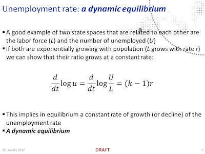
Because of that last point, I imagine that by "any unemployment rate can be an equilibrium" above he means any constant. Now it is true that in the dynamic equilibrium IE model, any given unemployment rate can be an equilibrium, but not any constant level. That's because the equilibrium is not in the level of unemployment, but its rate of change du/dt (or d/dt log u). This appears to hold empirically across several countries as I discuss in this presentation (pdf available at link) summarizing the results.

However!

There is a possibility to reconcile these views to some degree. The frequency and size of shocks to employment could be derived from an overlapping generations model (the current set of shocks is consistent with a Poisson process with time scale ~ 8 years, but maybe that 8 year time scale can be achieved with an OLG model). If those shocks are frequent enough and strong enough, compared to du/dt, then what you'd get is a degenerative state. Employment is then like Sisyphus ‒ every time du/dt brings the unemployment rate down, another asset price shock/employment shock happens. It could even be worse and the shock happens before Sisyphus has time to get back to the top. The employment level might look like this:

That is the employment population ratio for men; it appears to be hit with shock after shock before it has time to recover to its previous level [1]. It sinks lower and lower. Will this process continue? It seems unlikely to continue until the male labor force is completely unemployed, but the process by which it would stop is unclear.

Farmer's OLG models may provide an answer if the frequency of those shocks are related to the population's employment level. If the frequency decreases as the employment level falls, then there is a particular employment population ratio that is an equilibrium (and any EMPOP ratio can be an equilibrium) [2].

It's an interesting line of research, and I don't have all the answers. The latter piece after the "However!" is highly speculative. But blogs are for thinking out loud.

...

Update 5:30pm

This new post on matching functions is partially a follow-up to this post.

...

Footnotes:

[1] It appears that since the 1990s, women's employment may be subject to the same process.

[2] This also would provide an explanation of the so-called "Great Moderation" if the shock frequency is related to the employment population ratio. It peaked in 2000, and women's employment seems to reach dynamic equilibrium [1] in the 1990s.

An inflation forecast comparison update

I realized I hadn't updated the information equilibrium (IE) model comparison with the NY Fed DSGE model and the FOMC forecast since last August. Here is the most recent data (as of January 27th and 30th):

The IE model is still biased low [1], and the NY Fed DSGE model is biased high but we still can't really reject either model.

The FOMC was still very wrong back in March of 2014.

...

Footnotes:

[1] One thing I noticed is that since the IE model actually starts at the beginning of 2014 it did not see the boost in employment (and therefore NGDP) that came in mid-2014. That might explain the biased low inflation (as NGDP is a model input).

Dynamic equilibrium (presentation)

I put together some draft slides on dynamic equilibrium (here's a link to a pdf version, if my Google Drive settings are correct).

*  *  *

...

Update 29 January 2017

Here are the supporting post materials:

Unemployment equilibrium?

Dynamic unemployment equilibrium (and sunspots)

A dynamic equilibrium in JOLTS data?

Dynamic equilibrium: unemployment rate

Dynamic equilibrium: employment population ratio

Explaining the better wisdom of crowds

Exploring the state space.

Mark Thoma points us to MIT News about improving the wisdom of crowds:

Their method ... uses a technique the researchers call the “surprisingly popular” algorithm to better extract correct answers from large groups of people. ... 

The new method is simple. For a given question, people are asked two things: What they think the right answer is, and what they think popular opinion will be. The variation between the two aggregate responses indicates the correct answer. ... 

“The argument in this paper, in a very rough sense, is that people who expect to be in the minority deserve some extra attention,” ...

The interesting thing here is that this method essentially creates a measure of the degree of exploration of the "answer state space" (in economics: the opportunity set) as well as indicate possible strong "correlations". These are exactly the kinds of things you need to know in order to determine whether e.g. prediction markets are working.

Agents fully exploring the state space is critical to ideal information transfer in prediction markets. Correlations (agents cluster in one answer state) are one way to reduce information entropy; lack of exploration (no agents select particular states) is another.

In the example in the article, they ask the question "Is Philadelphia the capital of Pennsylvania?"

In a sense, the question itself sets up a correlation by anchoring Philadelphia in respondents' minds. Those that answer "no" indicate they have explored the state space (the set of all cities in Pennsylvania) -- they've considered other cities that might be the answer. Those that say others will answer "yes" give a measure of either a lack of exploration or a correlation. The people who expect to be in the minority deserve extra attention because they have more likely explored the state space.

Update 3 February 2017

Noah Smith has a Bloomberg View article about this result. What is interesting is that both his theories can be unified under a lack of state space exploration. Dunning-Kruger [pdf] is at its heart a lack of knowing there exist parts of the state space where you are wrong. You think most people will answer Philadelphia because you haven't considered that other people might consider that Harrisburg is the capital of Pennsylvania. As a non-expert, you probably haven't explored the same state space experts have. Noah's second theory is herd behavior; this is exactly the correlation I mention above.

...

Here's some more reading and background on information equilibrium, prediction markets, and state space exploration (what Jaynes called dither) at the links below. A slide package is here (the first few slides about Becker's "irrational" agents are relevant).

Is the market intelligent?

Thinking positive is thinking different

Corporate prediction markets aggregate random behavior

Jaynes on entropy in economics

...

PS I always get worried when information equilibrium "explains everything". It is true that this is an indicator that the theory is correct. However, it is also an indicator of an overactive left brain interpreter.

Dynamic equilibrium: employment population ratio

Part of doing research is just trying things. So I tried looking at the prime age employment-population ratio in terms of the dynamic information equilibrium model. It works a bit, but also fails a bit. And the failure might be interesting. It works well from the 1990s to the present:

However, before that time it's much more complex (I didn't even bother fitting the shocks, just extended the the fit to 1987-2017 back to the 1950s):

The interesting thing is that this was a period when many more people were entering the workforce in the US, especially women. In fact, if we look at men alone the dynamic equilibrium works great from the 1960s to the present:

Women entering the workforce is a strong non-equilibrium effect on the employment population ratio [see below], just like how women (potentially) impacted inflation (the high inflation in the 1970s was caused by demographics, not monetary policy).

...

Update 29 January 2017

John Handley thinks the projected increase in EMPOP is unlikely due to an aging population/demographic trend:

@jwhandley17 @infotranecon ignoring aging, participation is only about 1% below where it was in 2000, so further increases in EPOP unlikely pic.twitter.com/2MmwFG1aSv

— John Handleyハンドリージョン (@jwhandley17) January 29, 2017

Update 30 January 2017

Here is the view of women entering the workforce and reaching the dynamic equilibrium in the 1990s:

Rev. Bayes and the Dragon

Rev. Bayes is no St. George.

Francis Diebold brought up Bayesian versus frequentist interpretations of probability the other day and and I think Noah Smith retweeted it. It's actually a pretty funny framing of the argument. Diebold quotes a Bayesian econometrician who visited him in his office:

There must be something about Bayesian analysis that stifles creativity.  It seems that frequentists invent all the great stuff, and Bayesians just trail behind, telling them how to do it right.

I'm going to take issue with the last clause about doing it right. Now I've touched on this "debate" before, and I don't think I could have put it more perfectly than I put it then:

I've never been one to get into the Bayesian-frequentist argument, which much like the interpretations of quantum mechanics, seem to be a waste of my time (and are basically the same underlying issue). That it's a waste of my time does not imply it is a waste of your time if you happen to be a masochist who's into philosophical arguments that never go anywhere.

The thing is that there really isn't such a person as a "frequentist" who excludes Bayesian methods. At least I've never heard of such a person. I am fine with "frequentist" interpretations (which are just effective theories) as well "Bayesian" methods (which are just math). The issue as I see it is that there is just a subculture consisting of weird strict Bayesians versus everyone else.

When I read Diebold's post and Chris House's paper that he links called "Understanding Non-Bayesians", I thought I'd indulge my inner masochist and try to figure out exactly what Bayesians are on about.

The first thing to note is that Bayesian math is perfectly valid. The Bayesian approach is incredibly useful if you are updating pre-existing probabilities derived from older data using new data, or where you have a theoretical model of the prior probability. At least, that is how us "non-Bayesians" view it.

I think this probably falls under Chris House's description:

[To non-Bayesians] [t]he distinguishing feature of Bayesian inference then appears to be that Bayesians give explicit attention to non-flat priors that are based on subjective prior beliefs.

As I mentioned, I don't think the priors are always subjective. They can come from data that's been collected before or theoretical arguments. The weirdness (for me) comes in when the priors are subjective. What does it mean for a theory parameter to have a prior probability distribution before any data has been collected?

An excellent illustration of strict Bayesian weirdness is in a post I found in researching this topic called "Are you a Bayesian or a Frequentist? (Or Bayesian Statistics 101)". In the example worked out, a possibly unfair coin is flipped 14 times, coming up heads 10 times. The not "weird strict Bayesian" approach is to say 10/14 is an estimate of the unfair coin's probability p of coming up heads. The weird strict Bayesian approach is to stick in a prior probability distribution of that probability distribution parameter: P(p).

Now P(p) totally makes sense if you've encountered this coin before, or have some theoretical model of the center of mass of the coin (e.g. based on manufacturing processes). Even a so-called "frequentist" would approach the problem in exactly this way because Bayes' theorem is exactly what it says it is: a theorem.

However, imposing a non-uniform P(p) out of mathematical convenience or other subjective criteria effectively just increases the number of parameters in your model to include the parameters of the prior distribution. In the example, a beta distribution is used so now our model has two parameters (α and β giving us the distribution of p) instead of just one (p). If α and β summarize earlier data or our theoretical model gives us e.g. functions α(x) or β(x) of some parameter x (e.g. location of the center of mass), that's a different story. However, if you just posit a beta distribution then you're just adding parameters — which should be judged on information criteria like the AIC. Adding a non-flat Bayesian prior distribution actually makes the AIC worse in the coin example above unless you collect a few dozen more data points. There is also the problem of what P(p) even means if it is not derived from previous data or a theoretical model.

Chris House responds to this argument with tu quoque:

Though frequentist data analysis makes no explicit use of prior information [ed. not true per above], good applied work does use prior beliefs informally even if it is not explicitly Bayesian. Models are experimented with, and versions that allow reasonable interpretations of the estimated parameter values are favored. Lag lengths in dynamic models are experimented with, and shorter lag lengths are favored if longer ones add little explanatory power. These are reasonable ways to behave, but they are not “objective”.

In physics we have a heuristic we call "naturalness" with respect to theory parameters. However it is important to note that naturalness would never be used as a prior probability in estimating a parameter's likelihood, but rather as a rhetorical device hinting at a possible problem with the model. For example, the strong force is many orders of magnitude stronger than gravity. Physicists take that to mean there is probably something going on. We did not, however, incorporate a prior probability that the ratio should be natural in estimating the strengths of those forces.

Long lag lengths in House's hypothetical economic model that performs well against the empirical data (already requiring suspension of disbelief) might be "unnatural" based on the time scales in the theory (another thing economists haven't come to terms with), but that does not mean we should use that information to construct a prior that emphasizes shorter lags [1].

I would like to point out a nice concise point House makes:

A Bayesian perspective makes the entire shape of the likelihood in any sample directly interpretable, whereas a frequentist perspective has to focus on the large-sample behavior of the likelihood near its peak.

This is basically true, but also illustrates the issues with calling this "objective". The shape of that likelihood away from the peak is strongly dependent on the tails of the prior probability distribution, and the tails of probability distributions are notoriously hard to estimate. That is to say the Bayesian perspective makes the entire shape interpretable, but also strongly model-dependent and highly uncertain [2]. The so-called "frequentist" perspective is the practical one you should have: don't trust likelihoods except when you have large samples and then only near the peak. The rest of a probability distribution should come with a sign: Here be dragons.

...

Update 26 January 2017

This post on a specific prior producing a "counterintuitive" result is relevant.

...

Footnotes:

[1] This is not an argument against e.g. using the length of the available data as a prior. There you have a genuine information source (and Nyquist). I use the length of the available data to discount a lot of theories from Steve Keen's nonlinear models to Kondratiev waves and Minksy-like theories. Again, this is a rhetorical argument and I wouldn't compute a prior probability.

[2] This makes me think of the strange things that arise when economists talk about expectations at infinity (here, here) ‒ much like the tails of probability distributions, there be dragons in the infinite future.

Dynamic equilibrium in an agent based model?

A few months ago Ian Wright directed me to his Closed Social Architecture (CSA) agent-based model (ABM) based on random agent actions, and I attempted to describe it in terms of information equilibrium. I thought this might be an interesting test case for the dynamic unemployment equilibrium model.

So far, my initial poking around hasn't revealed anything conclusive. I thought I'd show you some graphs of the work in progress. The first graph is a fit to the ABM's unemployment rate u = U/(U + E) where U are the total number of unemployed and E are the total number of employed (so that U + E is the labor force). The second and third graphs are the information equilibrium relationships NGDP ⇄ P and NGDP ⇄ U that I found in the original link above (NGDP is total output and P is the profit level).