Update: Better title: "Angels dancing at the end of time"
In John Cochrane's paper [pdf] on neo-Fisherism, he posits that the representative household maximizes:
In John Cochrane's paper [pdf] on neo-Fisherism, he posits that the representative household maximizes:
E \left[ \sum_{t = 0}^{t = \infty} \beta^{t} u(c_{t}) \right]
$$
This is not an unusual equation and I'm not singling Cochrane out. It just happened to be the first place I saw this after writing this post. However, this is an interesting mathematical object. The only thing that makes the limit $t = \infty$ make sense is that there is an implicit time scale (call it $t_{\beta}$) over which the discount factor $\beta$ falls to zero. And $\beta$ exists in order to make the infinite sum convergent. There is also economic growth, so there is another timescale $t_{c}$ introduced through the consumption $c_{t}$. Let's pass through to continuous time and explicitly show our scales:
E \left[ \int_{0}^{\infty} dt \; \beta(t/t_{\beta}) \; u(c(t/t_{c})) \right]
$$
This has units of time, grows when $t_{\beta}$ grows (less discounting of the future) and gets smaller when $t_{c}$ grows (the economy is slower growing because the growth rate $g \sim 1/t_{c}$), so it must be [2]:
E \left[ \int_{0}^{\infty} dt \; \beta(t/t_{\beta}) \; u(c(t/t_{c})) \right]= \alpha \frac{t_{\beta}^{2}}{t_{c}}
$$
where $\alpha$ is some $o(1)$ constant dependent on the specific temporal shapes of the utility function and the discount factor [1].
The discount rate $1/t_{\beta}$ should be a deep parameter in the Lucas sense (based on how human behavior discounts the future) and the growth rate scale should be a deep parameter of the economy. So we should find the expected value at the top of this post depends primarily on the temporal shape of expectations (i.e. changes in $\alpha$).
It should therefore primarily depend on the temporal shape of expectations and discounting when exposed to shocks, since temporary shocks shouldn't change deep parameters (this is not a necessary restriction as we'll see below).
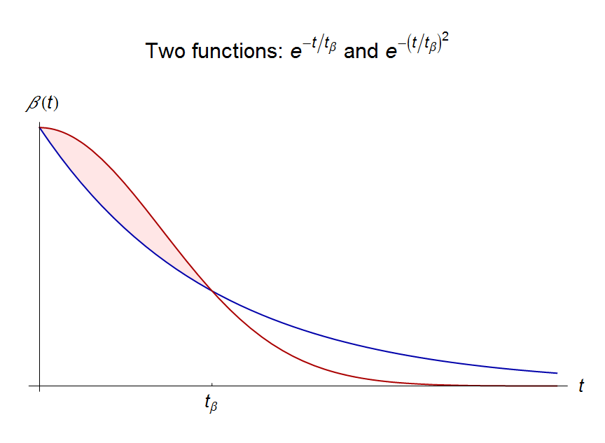
For example, I can cause the representative household's expected utility of consumption to fall in half by switching from $\beta \sim \exp -t/t_{\beta}$ [1] to $\beta \sim \exp -(t/t_{\beta})^{2}$. The difference comes from times $t > t_{\beta}$ -- far out in the tail of the distribution -- because for $t < t_{\beta}$ the second function actually has less discounting (the red curve is above the blue curve for small $t$, shaded region):
So you can see how expectations and discounting at 'infinity' can create results like Cochrane's and Woodford's.
In general, however, Cochrane's objective function maximized by the representative household (at the top of this post) gives us a really great way to organize several different takes on our current macro situation in the US:
- The neo-Fisherite view seems to be mostly about $\alpha$. I may be wrong about this, but that is what I am seeing.
- Both Paul Krugman's liquidity trap and Scott Sumner's NGDP are about changing the scale $t_{c}$ (Krugman says changing expected $t_{c}$ is hard without fiscal stimulus, Sumner says the central bank can set whatever expected $t_{c}$ it wants). Low interest rates are due to not just low growth in the short run (a change in $\alpha$), but low expected $t_{c}$.
- There don't appear to be any takes that directly modify the discounting scale $t_{\beta}$. However, since there are only two scales, it really only makes sense to talk about one relative to the other (i.e. $t_{c} > t_{\beta}$ or $t_{c} < t_{\beta}$). Therefore a change in $t_{\beta}$ could just be re-interpreted as a change in $t_{c}$.
Footnotes:
[1] Note that $\alpha = 1$ when $u(c) = \log(c)$, $c \sim \exp t/t_{c}$ and $\beta \sim \exp -t/t_{\beta}$.
[2] This is a fun trick we learn in physics called the "what else could it be?" argument (it's basically dimensional analysis). For example, the energy of an bound state of the Hydrogen atom, if $m_{p} \gg m_{e}$ kind of has to be
E \sim - k \alpha^{2} m_{e} + o(m_{e}/m_{p})
$$
where $k$ is some constant (turns out it's $k = 1/2$). The only energy scale is the mass of the electron (times $c^{2}$ but we're using 'natural' $\hbar = c = 1$ units, so mass is energy) and it's an (observable, not just an amplitude) electromagnetic interaction so you need two factors of $\alpha$ (coupling the electron to a photon and the photon to the proton). There is no other sensible combination that can come together to create something with the units of energy to be an energy eigenvalue. [$\alpha = e^{2}/4 \pi$ is the fine-structure constant -- there is a factor of $e$ (electric charge) coupling for the electron to the photon and the photon to the proton, and this is squared to get an observable, not an amplitude, proportional to $\alpha^{2}$]
No comments:
Post a Comment
Comments are welcome. Please see the Moderation and comment policy.
Also, try to avoid the use of dollar signs as they interfere with my setup of mathjax. I left it set up that way because I think this is funny for an economics blog. You can use € or £ instead.
Note: Only a member of this blog may post a comment.