Thursday, March 22, 2018

Effective information in complex models of the economy

Feedbacks in the economy (section)

Let me first say this is a great post from Sri Thiruvadanthai, and I largely agree with its recommendation to aim towards a resilient economic system rather than a stable one. And I would also agree that the idea that a single interest rate can stabilize the system (partially) pictured above from Sri's blog post is at best idealistic (at worst foolhardy) — if we viewed this system as a blueprint for a mathematical model. A mathematical model this complex is likely intractable as well, above and beyond using a single interest rate to stabilize it.

However, when I saw the diagram another diagram from Erik Hoel appeared in my head; I've placed Sri's diagram alongside Erik's:


Now it's true that Erik is talking about simple Markov chain models, but that might be interpreted as the limiting case of the information contained in asset prices, credit markets, economic activity, and benchmark rates [1]. In the limiting case, the "effective information" in this model for forming a causal explanation is basically zero. Another way to put it is that given enough feedbacks and connections between observables, your model becomes too complex to be useful to explain anything.

Now Erik's paper motivates so-called causal emergence: just as there are local minima of effective information, there are local maxima and we can think of the separation between these local maxima being related to scales in the theory. We understand chemistry at the atomic scale, but we understand biology at the cellular scale. Erik's conjecture is that this is a general property of causal descriptions of the universe from quarks to quantitative easing.

Now I understand this is just my opinion, but this is why I don't think a lot of "this is how the banking system actually works" will help us understand macroeconomics. Effective information and causal emergence is always at the forefront of my mind when I see descriptions like this (click to expand):


Such a model might well capture the details of the system, but might yield no insight as to how it actually works. Knowing what every neuron does could capture the phenomena of a brain system, but it probably won't yield answers to questions about consciousness or even how humans recognize objects in images [2].

And since the "emergent" but approximate descriptions with higher effective information at the higher scale don't have a 1-to-1 relationship with the model at the lower scale (they cannot because that 1-to-1 relationship could be used to translate one to the other implying that the effective information of the models at the two scales would be equal), there is no reason to expect the models to behave in ways interpretable in terms of the lower scale sub-units.

And now I come back to Sri's contention that changes to a single interest rate is unlikely to stabilize the system diagrammed above — especially if we think of interest rates in terms of the causal model above where we make some loose associate between raising interest rates and tightening monetary policy and damping economic activity.

I make the rather contrarian assertion in my blog post about monetary policy in the 80s that the increase in interest rates and "decisive action" from the Volcker Fed may well have mitigated the first 80s recession, but then the same stance caused the second. This is of course makes no sense on the surface (raising rates are both good and bad for the economy), but the feedbacks and strong coupling in Sri's diagram mean the system is probably so complex as to obliterate an obvious 1-to-1 relationship between the discount rate and economic activity.

However, it might have an effective description thought the causal emergence of politics and "Wall Street opinion". Volcker's "decisive action" in raising interest rates/targeting monetary aggregates was considered "good" because the government (Fed) was "doing something". The recessionary pressure ebbed, and the first recession faded. In the same way, quantitative easing might well have had "symbolic" effect in stopping the panic involved in the 2008 financial crisis. Volcker's and Bernanke's "decisive actions" might well have no sensible interpretation in terms of the underlying complex model at the lower scale. But at the macro scale, they may have helped.

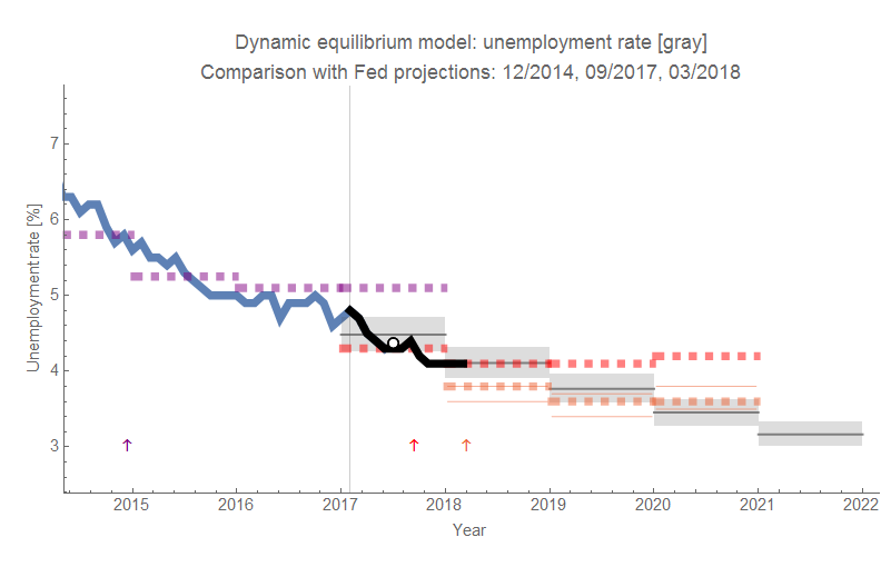
That's also how Volcker doing almost exactly the same thing again about a year later could cause a recession. Instead of being seen as "decisive action", the second surge in the discount rate was seen as the shock to future prices it was intended to be. In the underlying model, firms laid off workers and unemployment rose dramatically.

There's no single interest rate that stabilizes Sri's system, but one interest rate could be used as a focus for business sentiment and a complex signal of information.

Now there is a danger lurking in this kind of analysis because it leaves you vulnerable to "just so" stories at the higher scale, especially if you try an interpret things in terms of the complex underlying model. That's why models at the higher scale need to be constructed and compared to data. While we have physics models of protons, neutrons, and electrons, and use them to model atoms, we don't then say that chemistry involves complex interactions of atoms and use that to produce "just so" stories. We find empirical regularities in chemistry which have their own degrees of freedom like concentration and acidity. In some cases we can make direct connection between atoms and chemical processes, but other chemical processes are so complex that they're intractable in terms of atoms.

This also doesn't mean the lower scale model isn't useful. Sometimes the insight comes from the lower scale model. Sometimes you need to understand parts of it to do some financial engineering (such as Sri's contention to focus on making the system more resilient — solutions might come in terms of specific kinds of transactions or for particular assets). The "shadow banking system" comes to mind here; looking at the details might point out a particular danger. But the macro model might not need to know the details and interpreting the financial crisis in terms of a run on the shadow banking system with a Diamond-Dybvig model will have more effective information for macro policy than the details of collateralized debt obligations.


Footnotes:

[1] We can think of the nodes in that network themselves made up of more complex models as in another paper from Erik:


[2] There are similar contentions with machine learning where a system might be able to recognize any picture of a dog, but we won't really understand why at the level of nodes.

Wednesday, March 21, 2018

Fed revises its projections (again)


As unemployment continues to fall, the Fed has once again revised its projections downward [pdf]. The latest projection is in orange (the limits of the "central tendency" are now shown as thin lines). I added a white point with a black outline to show the 2017 average (which was exactly in line with the dynamic information equilibrium model from the beginning of 2017 as well as in line with the Fed's projection ... from September of 2017 with more than half the data for 2017 already available). The vintage of the Fed forecasts are indicated with arrows. The black line is the data that has come in after the dynamic equilibrium forecast was made.

One thing I did remove from this graph was the "longer run" forecast that is nebulous. I had put them down as happening in the year after the last forecasted year. But the Fed is wishy-washy about it, and I thought they were wrong enough already without adding in some vague "longer run" point. 


It's the 80s!

It's the 80s!
Do a lot of coke and vote for Ronald Reagan!
 
Mystery Science Theater 3000
David Andolfatto had a post asking the title question: What anchors inflation? The post represents a run-through of the monetarist view that the Volcker Fed anchored expectations through aggressive, manly credibility at the end of which Andolfatto asks whether fiscal policy had anything to do with it.

Now my contention is that in general from the 60s through the 90s a demographic wave of women entering the workforce was behind the existence of the Phillips curve so that recoveries and recessions were marked by rising and falling inflation. When this demographic wave crests in the late 90s, inflation and unemployment cease to have a relationship (because recoveries do not pull people into the labor force as they did before) resulting in our present day "price stability".

But I also believe that the actual process of recessions are largely social phenomena that can potentially be affected in their timing, severity and duration by political actions. That said: the 80s were complicated.

While Andolfatto claims that Fed policy under Volcker led to the recession, the recession (in terms of unemployment) had already begun in mid-1979 (first gray band in the graph below):


Additionally, there seem to be leading indicators ahead of the surge in unemployment (such as JOLTS measures unavailable at the time, or per a recent paper conceptions) so the recession had probably been building for several months before the unemployment rate spiked.

Oddly, a case can be made that the Fed's actions (based on the shock to the monetary base that Andolfatto uses) may have actually temporarily arrested the recession as the shock is ending as the shock to the monetary base is beginning. while this might be weird for a monetarist theory of recessions, it isn't weird for a social theory — the Fed was making announcements and people thought that something was being done. In the same way QE might have worked as symbolic action, Volcker's "decisive action" might also have symbolically alleviated fears.

Now some theories suggest (including the Wikipedia article on the tax cuts) that the "double dip" recession was caused by the deficit ballooning under the ERTA driving up interest rates. However, the ERTA is signed when the second shock is already underway and doesn't take effect until later anyway. It is possible that the deficits actually arrested the progress of the second shock or even lead to the third positive shock to employment in 1983 (this third shock may also be the rebound of the step response — a ripple following on the heel of the previous shock). The ERTA was also phased in, but some of the tax cuts were reversed with TEFRA (selected timings are indicated on the graph in red text/arrow).

Again, in general there seem to be indicators (e.g. JOLTS, as mentioned above) that lead spikes in unemployment by several months meaning this second recessions causes could go as far back as 1980.

Another possibility to consider is that the downturn in base growth was caused by the factors behind the recession, not monetary policy. But as I show the monetary base adjusted for reserve requirements (dashed line) takes a hit at the beginning of 1979. To try and disentangle the different timings, I looked at the currency component of the base, which also shows a downturn beginning in early 1979:


This expanded graph also shows a fourth shock to unemployment (or part of the continuing step response ripple), and a second shock to monetary base growth in 1984 (following the second hit to unemployment). The currency component shows a shock beginning even earlier than the recession shock (purple vs red bands). This coincides with the small shock to the adjusted base. However if this is used as evidence that monetary policy caused the recession, it completely discounts the entire "Volcker Fed" story as Volcker wasn't even nominated until about 6 months later in July 1979.

But there is other evidence that the recessionary indicators were building far before the downturn(s) in monetary base growth. The yield curve inverts in late 1978, and the stock market falls more than 10% in the last two weeks of October 1978. Oil prices are raised by two OPEC countries in early 1979.

All indications point to the first 1980s recession being a "normal" one caused by essentially a general downturn in business optimism. The cause of the second one is harder to pin down but is plausibly the one caused by the Volcker Fed's attempt to control inflation. One story told (e.g. on Wikipedia) is that high interest rates took a toll on housing [1] and manufacturing. There is some evidence of this: the discount rate drops after the first recession is declared to be over, however soon after the Fed begins to raise the discount rate and the effective Fed Funds rate (EFF) launches to over 20% around the time that Reagan takes office. With this spike, construction jobs cease their recovery and plummet again.

If the mechanics of the Phillips curve are as I described earlier, then the Fed did control inflation a bit by throwing people out of work. This inflation would begin to return  as soon as the recovery got underway; it was only the end of the demographic transition by the 90s that brought down trend inflation. In this model, the trade off was between a trend of slowly falling inflation and a temporary spell of rapidly falling inflation plus mass unemployment amid a trend of slowly falling inflation. It's possible the Fed's action arrested women's increasing labor force participation, but this seems unlikely as it hasn't resumed as the effects of the 1980s recession fade into history (i.e. the current "equilibrium" of ~10 percentage points higher employment population ratio for men than women more likely represents a new social or technology-driven [2] equilibrium).

So in the end, the 80s recessions are a jumble of "normal" factors and a possibly unethical macroeconomic experiment by the Fed based on incomplete and most likely incorrect theories. But the best story in terms of causality is that there was a normal short recession building in late 1978 that becomes the one NBER says started in January of 1980. As this recession begins to fade without bringing down inflation enough, the Fed hikes the discount rate initially to 13%, and then to 14% until employment starts to spike again. NBER says this one started in mid-1981, but in fact it started to get underway around the time the discount rate heads up to 13% in early 1981. Lower inflation was acheived via mass unemployment, but that lower inflation would have arrived by the late 80s or early 90s anyway due to the fading demographic shift. The end of that demographic shift is what appears to have "anchored" inflation, not Fed action or fiscal policy.

PS I used this paper [pdf] and this history article from the Fed for some of the dates and news events.

...

Footnotes

[1] I have a personal anecdote from this period. My parents moved to Houston in 1979 when my dad got a job in the oil industry. We spent the first few years in an apartment and two rented homes until they finally were able to get a mortgage for a house in 1983 when interest rates came back down a bit.

[2] Per this discussion, it is possible that post-war household production technology development was behind a shift of women into the labor force.

Friday, March 16, 2018

JOLTS data day!

Another month, another JOLTS data update from FRED. This time, we are getting a lot of data revisions, and the revisions to the quits rate are biased upward:


It turns out those data revisions erase most of the signs of a possible upcoming recession (i.e. the counterfactual) in both the quits rate and the hires rate (i.e. the original conditional forecast was more accurate). Click for larger versions:


The gray band indicates the shock counterfactual — which has completely collapsed back to the original forecast. There still is a deviation in the job openings rate, but this data is also noisier in general:


...

Update

A rehash of the analysis linked here tells us what my vague intuition claimed above — the data revisions have mostly eliminated the signs of recession in the joint probabilities of being further away from the original forecast (first graph is just probability that the distance from the forecast will be greater, second graph is the probability of at least one measure being further away [1]):


...

Footnotes:

[1] I.e. P(ΔJOR² + ΔQUR² + ΔHIR² > Δ²) for the next point where Δ² is the distance for the latest point versus P(ΔJOR > Δ₁ || ΔQUR > Δ₂ || ΔHIR > Δ₃) for the next point where  Δ = (Δ₁, ΔΔ).

Okun's law and the labor force

I was curious about how the dynamic information equilibrium model of RGDP (described in a presentation/Twitter talk available here) matched up with an equivalent model of employment L (FRED PAYEMS) — they should to some degree because of Okun's law (for a more formal version in terms of information equilibrium "quantity theory of labor" see here). However a naive application doesn't work very well for basically the same reason that the "quantity theory of labor and capital" outperforms the "quantity theory of labor": there is effectively a dynamic equilibrium shock that is different between labor and NGDP that is compensated by the use of capital in the former of the two models. Here's that naive version:


So I tried to correct for this by combining the dynamic equilibrium model for the civilian labor force (CLF) and another one for the "employment rate", i.e. L/CLF. Here is the L/CLF model:


Multiplying by the dynamic equilibrium model for CLF (see e.g. here), we get a decent model of the employment level:

One big deviation is due to the fact that I am treating the 1980s recessions as a single recession (and there is a concomitant step response [1]). This won't be terribly relevant to the analysis here. The next thing to do is put the RGDP growth rate model (red) and the PAYEMS growth rate model (green) on a graph together:


These should be the identical models if Okun's law is a perfect description. As you can see, RGDP growth over estimates PAYEMS growth, specifically in the 90s and 2000s booms (dot-com and housing "bubbles") [2]. The thing is that the late 90s and 2000s is precisely where the RGDP and PAYEMS models are working best, so that deviations there imply that Okun's law is at best an approximation. It makes sense — increased real output during asset bubbles shouldn't be as closely linked to labor market booms.

The models in the "Phillips curve era" from the 60s through the 90s shouldn't exactly match up either because the oscillations due to RGDP are due to oscillations in the price level that precede the shocks to employment as can be seen in the graph above as well as in a chart from my presentation on macro trends:


All of this points to Okun's law being an approximation due to the fact that RGDP and PAYEMS are going to be highly correlated because a) recessions are where employment and output fall, and b) between recessions you usually have growth. In the past, when the Phillips curve was in full effect, the correlation was even better (the Phillips curve is a direct link between employment and inflation, the latter being essential to real output). This link persists through the entire business cycle in that era. More recently when recessions and output seem to be driven by exogenous factors to the labor market (e.g. commodity booms in Australia, asset booms in the US), the connection between the two variables is primarily via the recession.

I'm still trying to make sense of this myself, so I apologize if this comes across as a word salad. There does seem to be an effective macro theory consisting of Okun's law and the Phillips curve valid from the 60s through the 90s. More recently, a different — and less understood —effective theory has taken over.

...

Footnotes:

[1] Speculating, but maybe the fading of the step response is linked to the fading of the Phillips curve I mention in my presentation?

[2] There are also significant deviations between the RGDP model and the RGDP data (faint red on the graph) in the case of the "Phillips curve" recessions of the 70s, 80s, and 90s. These could potentially be connected to the step response noted in footnote [1]. 

Thursday, March 15, 2018

Why I dislike the map metaphor in economics

voronoiUSA

While the thesis of this essay by Esteban Ortiz-Ospina is fine, the map metaphor needs to go. Map metaphor?
The different views on what economists actually do can be nicely captured in metaphors. I find the cartography metaphor spot on: economists try to create and use maps to navigate the world of human choices. 
If economists are cartographers, then economic models are their maps. Models, just like maps, make assumptions to abstract from unnecessary detail and show you the way. 
Different maps are helpful in different situations. ... If you are hiking in the Alps and you want to find your way, you will want a map that gives you a simplified perspective of the terrain ... A map with elevation contour lines will be very helpful. 
On the other hand, if you are an engineer trying to calibrate the compass in an airplane, ... you’ll want ... a map that highlights magnetic variation by showing you isogonic lines.
It's a common metaphor. Paul Romer used the metaphor in one of his critiques of economics. Alan Greenspan used it as the title of a bookThe metaphor derives from Alfred Korzybski, who was as best I can tell kind of a philosopher. The metaphor has its use [1], but I think its use in macroeconomics is problematic. 

The reason? An elevation map is still an empirically accurate description of elevation; a magnetic map is still an empirically accurate description of the magnetic field; Romer's subway map is still an empirically accurate description of the network topology. And in the case of various projections of the Earth's surface, we know how those maps distort the other variables! A DSGE model (to pick on one example) may be an abstract map of a macroeconomy, but it's not an empirically accurate one [pdf].

Of course the abstraction of that DSGE model (or other models) is then used as a rationale for the lack of empirical accuracy, making the whole argument circular [2]. 
Economist: Abstractions are useful for the variables they explain. 
Critic: But they don't explain the data for even those variables. 
Economist: It's an abstraction, so it doesn't have to explain data.
Now Olivier Blanchard would argue that I'm not talking about data for the right variables for the model in question (e.g. DSGE models don't forecast, they tell us about policy choices). However, 1) it is bad methodology to make ad hoc declarations about which data a model can be tested on, and 2) this doesn't make any sense in the particular case of forecasting as I extensively discussed in an earlier post [3].

The map metaphor is only useful if your map is accurate for the variables it isn't abstracting. Now this isn't to say "econ is wrong LOL", but is a critique of how much economists (in particular macroeconomists) claim to understand. I'm not just talking about the econ blogs, news media, or "pop economics". David Romer's Advanced Macroeconomics has lots of abstract models, but little to no references to empirical data. It's written like a classical mechanics textbook, but without the hundreds of years of empirical success (and known failures!) of Newton's laws. 

I'm in the process of moving and came across my old copy of Cahn and Goldhaber's The Experimental Foundations of Particle Physics. While a lot of quantum field theory and quantum mechanics lectures in physics are pretty heavy on the theory and math, there are also classes on the empirical successes of those theories. C&G is basically a collection of the original papers discovering the effects (or confirming the predictions) that are explained with theory. While Romer's book might be the macro equivalent of Weinberg's The Quantum Theory of Fields, there is no book called "The Empirical Foundations of Macro Models".

This is not to say macroeconomics should have these things right now. In fact, it shouldn't have an analog of either Weinberg or C&G. Its modern manifestation is still a nascent field (the existence of a JEL code for macroeconomics is only a recent development as documented by Beatrice Cherrier), and while Adam Smith wrote about the "wealth of nations" even the data macro relies didn't start to be systematically collected until after the Great Depression. Physics has an almost 300 year jump on economics in that sense. I really have to say that is part of the allure for me. Going into physics, so much stuff has been figured out already. Macroeconomics seems a wide open, un-mapped frontier by comparison [4]. And that's why I dislike the map metaphor — there really aren't any accurate maps yet [5].

...

Update

PS There is a paper [pdf] by Hansen and Heckman called The Empirical Foundations of Calibration, but that's 1) a paper, and 2) more of an attempt to motivate a case for calibration as an empirical approach. Calibration (and method of moments) is quite a bit less rigorous than validation. There is a University of Copenhagen course called Theoretical and Empirical Foundations of DSGE Modeling that appears to relegate empirical evidence in favor of the models to a guest lecture at the end of the course. They do teach students to "Have knowledge of the main empirical methodologies used to validate DSGE models", but that just seems to be how one would go about validating them.

...

Footnotes:

[1] However, adherence to this metaphor would have prevented physicists from predicting the existence of antimatter, discovering the cosmological constant, understanding renormalization, coming up with supersymmetry, and finding the Higgs boson. These are all things that are based on taking the "map" (the mathematical theory) so seriously that one reifies  model elements to the point of experimentally validating them — or at least attempting to do so. Dirac's equation for electrons with spin had a second solution with the same mass and opposite charge: the anti-electron. Einstein's equations for general relativity in their most general form contain a constant (that Einstein declared to be his worst mistake; I do wish he had seen his "mistake" empirically validated). Renormalization sometimes introduces additional scales, such as the QCD scale, that are very important. Supersymmetry is required to make string theory make sense, and the Higgs boson was just a particular model mechanism to give mass to the W and Z bosons — it didn't have to be there (there are other "Higgs-less" theories).

[2] This is part of the critique of Pfleiderer's"chameleon models". Abstractions are made and used to make real world policy recommendations. When those abstractions fail to comport with real world data, the models are defended by saying they are abstractions.

[3] I'm also not sure those DSGE models are empirically accurate in modeling the distortions due to policy either.

[4] It being a "social" science, it may well be doomed to being wide open because no empirically accurate models will ever be found. You will pay the price for your lack of vision!

[5] For the record, I think there are some empirical regularities and some simple models that are probably fine (Okun's law comes to mind). But not enough to fill up a textbook, unless it's dedicated to e.g. VARs.

Wednesday, March 14, 2018

Employment growth and wages

Kevin Drum posted a blog post wherein he supports the bold claim of the title "Employment Growth Has No Effect on Blue-Collar Wages". In fact, I think Drum himself thinks the claim is a bit too bold:
I would think that two years of employment growth—no matter where it’s starting from—would lead to at least some growth in blue-collar wages. But the correlation is actually slightly negative. This seems odd. What do you think the reason could be? Is prime-age employment completely disconnected from blue-collar employment? Or is it something else?
His conclusion is actually supported by the data he presents. However the data he presents is incredibly noisy (wage data, especially after being adjusted for inflation & employment population ratio growth data), so some back of the envelope chartblogging won't really see it. You need a model.

So I applied the dynamic information equilibrium model (described in detail in my paper). Note that the wage growth data is extremely noisy. There is less noisy data from ATL Fed that I blogged about awhile ago; here they are side by side (click for high resolution):


The (prime age) employment-population ratio (EPOP) model is less noisy (the derivative linked above is still pretty noisy):


If we put these together in a macroeconomic "seismograph" where we show the shocks to the dynamic equilibrium, we can see these measures all show the same general structure (click for higher resolution):


We can (barely) infer a possible causal relationship where EPOP drives wage growth (negative shocks to EPOP precede negative shocks to wage growth). This is not to say this is absolutely the true causal relationship, just that the other direction (wage growth cause EPOP changes) is basically rejected by this data. Plotting them versus time on the same graph lets us see that they're basically the same (I also show real wages deflated by the GDP deflator and CPI):


This relationship would not be visible were we not able to extract the trend using the dynamic information equilibrium model:


Tuesday, March 13, 2018

Black labor force participation

While women entering the work force was the larger effect (almost doubling from 30% in the 1950s to almost 60% at its peak), another social transition was the increase in black labor force participation after the anti-discrimination laws of the 1960s.

Since it was a smaller effect — rising about 10% [1] in the same period women's labor force participation rose about 50%, and black women's participation rose 30% [2] — the business cycle fluctuations are more readily seen. And from that we can gather a bit more evidence about the effect of labor force participation on inflation. Here's the model result:


Before 2000, between recessions there is a positive shock to black labor force participation (the sum of these shocks is effectively equivalent to the broad shock to women's labor force participation). One way to interpret this is that while the social transition is happening, the booms of the business cycle correspond to people entering the labor force at an increased rate. After 2000, however, black labor force participation shows roughly the same structure as overall participation, men's participation, and women's participation —  participation falls after recessions and no inter-recessionary boom.

The other noticeable effect is the labor force bump comes before bumps in inflation [3]:


This provides further evidence that inflation may be a phenomenon of the labor force (i.e. not monetary), and its recent sub-target performance may be due to the end of the demographic transition and its concurrent increase in labor force participation.

Note that I'm not claiming increases in black labor force participation increase inflation, but rather that general increases in labor force participation increase inflation. Looking at black labor force participation helps make the causal structure of the shocks more clear because women's participation is increasing too fast to see the business cycles as clearly.

...

PS

One of the things I found interesting about modeling this data is that the entropy minimization process was not completely conclusive:


One minimum is lower than the other, but the resulting model — while simpler — makes less sense than the one described above. 


Black labor force declines in this version are endemic, and it's only kept from falling to zero by booms that come between recessions. Recessions effective end these booms and return black labor force participation to its typical state of decline. This would be hard to reconcile with basic intuition (shouldn't labor force participation flag after a recession?), but also impossible to reconcile with the relative similarity in the structure of black and white unemployment rates.

That's why I chose the other minimum despite it being only a local minimum, not global.

...

Footnotes:

[1] Not 10 percentage points, but 10% from about 60% to about 66%.

[2] In fact, black men's labor force participation fell during this time, so the rise overall black labor force participation can mostly be attributed to black women entering the labor force.

[3] This would predict a positive shock in labor force participation in the early 70s before the beginning of the available data.

CPI data and the end of "lowflation"

The latest CPI data is out for the US, and I think it's looking like the recent shock (2014-2015) parameters were a bit off (since it was still ongoing at the time). While this has negligible effect on the continuously compounded annual rate of inflation (instantaneous logarithmic derivative), it produces a noticeable effect (within the error) on the level and when measured year-over-year [1]. Here's the instantaneous inflation measure:


And here are the year-over-year and level measures:


The original estimates of the shock parameters were

a₀ = 0.088 ± 0.026
y₀ = 2015.06 ± 0.90
b₀ = 1.27 ± 0.41 [y]

That b₀ corresponds to a duration of 4.4 + 1.4 years, which means the shock was still ongoing when the forecast was made in early 2017. The new estimate (shown as a dashed line in the graphs) has parameters

a₀ = 0.078 ± 0.009
y₀ = 2014.73 ± 0.41
b₀ = 1.16 ± 0.27 [y]

which are all within the error bars on the original estimate (the new errors are all approximately cut in half as well). So we can see this as a true refinement. This new b₀ corresponds to a duration of 4.1 + 0.9 years. The shock "began" (inasmuch as you can cite a "beginning") in late 2012 or 2013 and "ended" in late 2016 or 2017. This period of "lowflation" is associated with the negative shock to the labor force after the Great Recession and appears to be ending (or has already ended as of last year per these new parameter estimates).

...

Footnotes:

[1] The CPI level accumulates (integrates) the error, while the year-over-year measure amplifies it (x + δx)/(y + δy).

Monday, March 12, 2018

New forecast comparisons to track (US output and inflation)

After wrapping up the previous head-to-head forecast between the NY Fed DSGE model and a model using the information equilibrium framework, I'm starting up a new comparison between their DSGE model and the dynamic information equilibrium model (also shown at the first link and described here).

These are the forecasts for output (4Q growth in RGDP) and inflation (4Q growth in core PCE inflation); I'm showing the 50% and 90% confidence intervals (the original FRB NY graphs show more intervals):


Ergodicity!

Roger Farmer has an interesting summary of the meeting he had as part of the Rebuilding Macroeconomics project. Several points were great. First, a couple of quotes:
At each level of aggregation, natural scientists have learned that they must use new theories to understand emergent properties that arise from the interactions of constituent parts.
I would only say that instead of "they must use", I would write "it is more efficient to use". The people that do direct aggregation are doing valuable work, and there are zero cases in natural science where they have given up aggregation for emergent theories. Lattice QCD has been validating the effective nuclear theories, and neuroscientists haven't given up on explaining brain function in terms of neurons. Roger probably makes the statement the way he does because of the "hegemony of microfoundations" in macro that seemed to invalidate aggregate approaches that weren't derived from 'rational' individual behavior.

I liked this quote as well:
Some have argued that the social world, like the weather, is obviously governed by chaotic processes; the so-called butterfly effect. What I have learned in my discussions with the applied mathematicians and physicists who attended our meeting, is that the natural world is far less predictable than that. It is not just the variables themselves that evolve in non-linear chaotic ways; it is the probabilities that govern this evolution.
One thing to note is that the chaos in dynamical systems is a kind of "precision chaos" that differs from the colloquial use of the word chaos. You can't necessarily cobble together a nonlinear circuit that automatically manifests it without some fine tuning [1], and adding noise can easily disrupt any patterns.

Roger says that the theme of the meeting seemed to be that macroeconomics needs to think about non-ergodicity. Ergodicity has a slightly different meaning in statistics (Roger's sense) than in physics, but the basic idea is that it is an assumption about the representativeness of samples (i.e. that they are representative) in forming aggregate measures. The specific sense Roger's using it is that obesrvation of a random process over a long enough time will produce an estimate of the random process's parameters (that can be used for e.g. forecasting). As a slogan, non-ergocity is inherent in the statement that past performance is not guarantee of future returns.

Ergodicity is not always a good assumption, but Roger's characterization is a bit of an exaggeration:
... agent-based modellers and the econo-physicists are perplexed that anyone would imagine that ergodicity would be a good characterization of the social world when it was abandoned in the physical sciences decades ago.
We still make assumptions of ergodicity, just not in all problems. That's the key, and that's where I differ from Roger's opinion.

First, a bit of philosophy. Ergodicity is a property of aggregating the underlying degrees of freedom (agents, process states, etc), but not a property of the aggregate itself. Ergodicity is used to aggregate atoms in statistical mechanics to derive the ideal gas law. The statistical mechanics is ergodic, not the emergent ideal gas law. If we have that emergent economic theory Roger mentions in the quote at the top of this post, the theory is neither ergodic nor non-ergodic (unless it is further aggregated at a higher level ... e.g. ergodic neurons aggregate to brains which are non-ergodic when aggregated to an economy).
Since ergodicity is a property of the agents and the aggregation process, we really have only one of two ways to determine whether non-ergodicity is important:
  1. Aggregate some non-ergodic processes/theory into an empirically successful macro theory
  2. Have a really good (empirically accurate) theory of the underlying process or agents that shows to be non-ergodic
In the first case, the agents or processes don't even have to be realistic (macro success is sufficient). The second case is the one used in a lot of natural sciences where we tend to have really good "agent" models (e.g. atoms in physics).

The problem with Roger saying macro "needs to deal with" non-ergodicity is that we have neither good agent models nor a successful macro theory made up of non-ergodic processes. Therefore we have no idea whether macro is non-ergodic or not. Our inability to forecast could just be because we are wrong about how economies work. If you can't predict inflation, you shouldn't jump to inflation being a non-ergodic process. Sure, someone can and should try that, but others should question whether more basic aspects of the model are correct (such as the correct input variables).

Like "complexity" (or any other ingredient you might think "needs" to be in macroeconomic theory), the proof of the relevance of non-ergodicity is in empirically successful models that incorporate it.

...

PS In his post, Roger cites Mark Buchanan as an econophysicist who has questioned ergodicity. I don't know if Buchanan was at the meeting or is any part of the source of this emphasis on non-ergodicity. Regardless, Buchanan cites Ole Peters as his impetus for thinking about non-ergodicity (a collection of links here).

However Peters paper on non-ergodicity represents a mathematical slight of hand, and not an actual demonstration of non-ergodicity. It's an apples to oranges comparison of a geometric mean to a arithmetic mean that I talk about in these two posts:


If you enjoy math jokes, you might like the first post. The second post goes into more detail about how the infinity is made to magically vanish in the case of a geometric mean.
...

Footnotes

[1] An implementation here of Chua's circuit requires humans to fine-tune a couple of resistors to achieve chaotic behavior. The models developed by Steve Keen are basically nonlinear circuits like this — I am highly doubtful macroeconomies run with this kind of precision.

Friday, March 9, 2018

Vestigial monetarism: Japan edition

A little over a month ago, I wrote a post about how I was laying the last of my "vestigial monetarism" to rest. I didn't explicitly talk about it, but that should also include the monetary model of Japan's consumer price index (last updated here I believe). 

The most recent data (adjusting for the VAT) is actually still consistent with the model:


Unlike a lot of other macro models, this one didn't "die" (H/T Noah Smith) because of Japan but rather because the dynamic equilibrium model of the US data was far more convincing than the equivalent US monetary model (read more about my thinking here).

However, I'll continue to track the dynamic equilibrium model of Japan's CPI (which is (also) doing fine):


Validating employment situation forecasts

The latest employment situation data is out and the latest data is still in line with the forecasts (previous update was here). I've been following the unemployment rate model for over a year now. A lot of people are talking about the increase in labor force participation (there's an especially big spike in "prime age" CLF, but even that spike is consistent with the expected fluctuations in the model. I'll just present the graphs in a gallery (the new data is in black, and the two comparisons are versus various vintages of the FRB SF forecasts and the Fed FOMC forecasts — as always, click for full resolution).

There are two models of the CLF participation rate (one posits an additional shock for reasons explained in a post here):


Also, here's the novel Beveridge-like curve between CLF participation and unemployment discussed in that same post:


And finally, here are the unemployment rate forecast graphs (this model was discussed in my recent paper up on SSRN):


Thursday, March 8, 2018

Trends in macro observables: twitter talk and pdf download

I did another "twitter talk" (see here); in honor of International Women's Day, the subject was the demographic shift of women into the workforce and other trends in macro observables. A pdf can be downloaded here (let me know if my Google Drive settings aren't working for you).


Wednesday, March 7, 2018

Economic growth in Australia 1960-present


I saw the chart above on Twitter; it made me want to try this analysis using the dynamic information equilibrium model for Australia to see if I could understand the near constant decline in RGDP growth since the early 2000s because it looked very odd from a dynamic equilibrium standpoint. The data I have from FRED for Australia is a bit noisier than the US and UK data so there is the oddity that the model sees the Great Recession as more of a statistical fluctuation than a shock. Here are the models of NGDP and the GDP deflator (click for full resolution):


The dynamic equilibria are 5.8% NGDP growth and 2.8% inflation, resulting in 3%. The demographic shift (discussed below) is highlighted in gray. And here is how they combine as RGDP growth (click for full resolution):


Overall the picture for Australia is approximately the same as for the US and UK: a "Phillips curve era" accompanied by a demographic transition in the mid-to-late 1970s and a more recent era with sparser shocks. I hesitate to give it the same "asset bubble era" label I gave the US and UK because it seems more associated with the "commodity boom" of the 2000s (centered in 2006). There was also a major (nominal) commodities bust centered in 2014, but as it was accompanied by a nearly equal negative shock to inflation it turns out to be a wash in RGDP. In fact both shocks in the post-Phillips curve era effectively combine to create a slow steady decline in RGDP. Here is the dynamic equilibrium model version of the 10-year average RGDP growth graph at the top of this post (click for full resolution):


While the forecast looks a bit strange, it is entirely due to the backward-looking 10 year average (which also makes the 10 year average growth rate higher than the continuously compounded rate about at 3.6%) and in the continuously compounded rate of change we have a simple return to about 3% RGDP growth following the "commodity bust".

Australia is frequenty noted for its long recession-free streak following its early 90s recession (which in fact has almost the exact same structure as the "Lawson boom" — and subsequent bust — in the UK data), with some attributing it to effective monetary policy. I'd attribute it to the high rate of NGDP and RGDP growth (likely stemming from a high rate of population growth, about double the US) that makes even large negative shocks like the Great Recession insufficient to generate more than a single quarter of negative growth (it's effectively interpreted by the model as the ending of the "commodity boom" than its own "shock"). But also the shocks to nominal growth and inflation are both broader and more correlated for Australia resulting in less jagged RGDP growth (which tends to be associated with recessions). This correlation may well be due to the fact that the nominal growth is associated with commodities rather than financial and/or housing asset bubbles in the UK and US (Minsky!). Although housing prices appear to have been rising in Australia (only to begin to decelerate more recently), there does not appear to be a separate "housing bubble" effect readily visible in the data — maybe housing prices were associated with the commodities boom rather than an independent phenomenon (for US readers, think North Dakota housing prices in the 2010s rather than Florida/Arizona in the 2000s)?

But the broad themes here are similar to the US and UK: a big demographic shift has ended (and with it, high growth), and we've entered an era of booms and busts and more moderate growth.