Why focus on supply and demand?

Jamie has a couple of excellent comments on my previous post and I thought I'd turn the response into a full post (as I've done before). I broke my response up into two pieces more or less corresponding to the two comments with 'short answers' for the titles. I also left (i.e. will have left, after I write this) some responses to some of the side questions on the comments themselves.

I. Supply and demand as entropic force free-body diagrams

Jamie's first comment asks why I focus on supply and demand (my derivation of supply and demand diagrams is probably one of the most linked-to posts on this blog), especially in macroeconomics, when -- and I am paraphrasing here -- the counterfactual points along the curves that are not realized are unobservable.

First, there are some practical reasons. You can't get very far winning people over to your view if you start from the perspective that their entire education in their field was for naught. I try to make a connection with mainstream results -- where they are similar -- as a method of persuasion. I also try to use the language of the field where possible. My primary purpose is so that I can communicate with economists. [1]

Additionally, in the specific case of supply and demand, the concept been around for 200+ years and is still considered a good guiding principal by economists. There is probably something to it, even if it is just an approximation.

And it turns out the idea of information equilibrium when you hold one of the quantities constant leads to the logic of a supply and demand diagram. A good analogy for a supply and demand diagram is a free-body diagram from introductory physics classes.

In physics we learn F = ma and one way to figure out the acceleration (a) is to figure out all of the forces acting on an object, which is done with a free body diagram like this one from wikimedia commons:

Two of these (psuedo)forces, friction (f) and the normal force (N) are not directly observable on their own -- the force of gravity (or some other force) has to be acting in the opposite direction.

A supply and demand diagram is a bit like a free-body diagram, but for entropic forces. Take osmosis for example. Adding salt or water to either side of the semi-permeable membrane is a bit like shifting supply and demand curves with the osmotic pressure going up and down. When you shift one of the curves, your equilibrium price (pressure) travels along the other curve, and even though we may not add salt or water, the unobserved parts of these curves exist and are useful theoretical constructs.

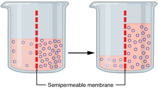
Osmosis.

Additionally, Smolin's advice:

"The observables of economics are accounting and other records. One should then try to construct a theory of economics that involves only observables. The importance of this kind of operational principle in physics and other sciences have been paramount"

refers to something a bit more technical than constructing a theory only using observable quantities. Smolin, a theoretical physicist, is not arguing that the idea of a wavefunction (not observable) should be left out quantum mechanics! In fact, in Smolin's view, the sale price of e.g. an iPad is not really an observable:

"In physics we have a basic rule which is that observables are always expressible as ratios of two quantities expressed in the same units, so they are a pure number. Applied to economics, this rule suggests that decisions should not be based on the units or currencies prices are expressed in."

What Smolin is arguing (I believe -- his two statements about observables are somewhat contradictory) is that we should restrict the inputs and outputs of economic theories to observable quantities (in the same way that that the inputs and outputs of quantum field theory are restricted to things that can be measured in a lab -- the Ψ's are in the theory, but aren't directly observable). Specifically, Smolin mentions utility which I think is the prime example (I would add expectations as well). Utility functions cannot be observed so there are things like the axiom of revealed preference -- which turns out to be equivalent (via Afriat’s theorem) to the idea that utility functions should be observable in Smolin's view!

To bring it back to the osmosis example, the movements of the water molecules are unobservable in principle. It takes kT log 2 units of energy to erase one bit of randomness, so observing the velocities of all the molecules would raise the temperature of the system and impact the experiment [2]. But we wouldn't think we should leave the idea of molecules out of a description of osmosis.

It is true that you can understand the information transfer framework without introducing supply and demand diagrams -- for example, an ideal gas is described by the exact same mathematics, but we don't draw supply and demand diagrams (PV diagrams are a more relevant way of discussing gasses). But sometimes these diagrams are a useful tool for explanations when there is a bunch of stuff going on or to appeal to intuition of the reader. Here is a good example.

Essentially, I focus on supply and demand because it is part of the language we've ended up with in the intellectual history of economics that matches up best with the entropic forces (the 'invisible hand') described by the information transfer model.

II. With entropic forces, causality goes both ways

Jamie's second comment asks why I like forecasting (which has a short answer -- I'm a scientist, and the only way you can guarantee your model didn't have access to a given data set is if it comes from the future), but primarily asks about causality and uses the example of driving a car. I think this question really hits at the heart of different ways of thinking about economics:

Which of the following statements is more accurate?

1) An increase in fuel [supplied] causes the car to travel further
2) An increase in the use of the car for travel causes an increase in the fuel [used].

Jamie, logically, says (2) is the more sensible sentence from a causality standpoint. I'd agree!

The utility-based microeconomic theory (that "incentives matter") says that (2) is true, too. Additional demand increases the price, that incentivizes additional fuel production. However, this view also says that an increase in the fuel supply (1) lowers its price and that makes more people buy more fuel. Now this idea is not only that more people can afford fuel at a lower price, or finally afford as much as they need, but that lowering the price incentivizes additional consumption ... like a moth to flame. Jamie and I both have a problem with this view. Lowering the gas price doesn't make me want to drive more. I didn't look at the gas price at the pump I went to here in New Mexico (I'm on work travel again), see that it was almost two bucks a gallon (I haven't seen prices that cheap since the 1990s) and feel the urge to buy more gas than I needed or drive more than I have to.

Despite my problem with this microeconomic view, I still think it gets the result correct, just not for the right reasons. The problem with the micro viewpoint in the previous paragraph is that is tries to assign a microeconomic explanation for an entropic force. I've talked about this before here. As an analogy in physics, it is like coming up with a microscopic force that causes a single water molecule to undergo osmosis or a single glue molecule to be sticky. There is no such force [3]. Water molecules end up on one side or the other of a semi-permeable membrane because they are more likely, given all of the places they could be, to be there.

In some cases, it is possible to invent microscopic forces that save the phenomena, but they're not real. I think a good case in economics is Calvo pricing. In order to produce microfounded models with sticky prices, economists invent a "Calvo fairy" that randomly goes around and with a touch of its wand, lets a firm raise or lower their prices. In the information transfer model, nominal rigidity is an entropic force -- there is no microeconomic explanation. Nothing prevents firms from changing their prices, it's just overwhelmingly unlikely that they all do it in a particular way (unless there is a recession).

As in the case of osmosis, adding more salt to right side "causes" the water to move over to the right side and adding more water to the left side "causes" more water to move over to the right side. But there is no microscopic force acting on the water molecules to move them. It is just becomes overwhelmingly more probable to find the system in the new state. If you had only a few water molecules and sodium and chloride ions, the probability wouldn't be as overwhelming, and you could in fact see things go the "wrong" way.

Jamie brings up the question of whether adding money (or expectations of money) to the economy causes NGDP to grow (the monetarist viewpoint) or an increase in NGDP (via e.g. government spending) causes the money supply to grow. The answer to this in the information transfer model is "yes" [4]. That is to say:

• Adding money to the economy makes it more likely that the economy will randomly happen upon a state that has higher NGDP [4]. That is to say, there is an entropic force that pushes the economy to higher NGDP [4]. This brings M and NGDP into information equilibrium.
• Adding NGDP to the economy creates an entropic force that results in more money being printed (more people go to ATMs, the banks ask for cash from their reserves, and the Fed asks the Treasury to print it up). If that money isn't printed (because the central bank says "no"), M and NGDP will be out of equilibrium. If that happens, NGDP can fall back suddenly, causing a recession.

I talked about causality more awhile ago here, and I'm saying essentially the same thing now (the linked post uses interest rates as the example). In the end, the information equilibrium picture is a very different view of economics from any I've seen out there.

This is not to say that an agent-based approach that simulates millions of micro interactions won't end up with the correct theory. It totally could! A simulation that models all the velocities and interactions of the molecules in a gas will come up with the ideal gas law. The thing is that the specific list of causes and effects in all of those microscopic interactions fall away -- the ideal gas law doesn't depend on the details of the molecules except as a single number (the ideal gas constant).

The information transfer model posits that the same goes for macroeconomics.

Footnotes:

[1] For example, the term "liquidity trap" (frequently appearing in quotation marks on this blog) is really not very accurate. Calling it a "trap" makes it seem like it has a rapid onset (it does not -- you just notice it rapidly when the first large economic shock strikes when inflation is low). And it has nothing to do with liquidity preference either. Most accurately, a liquidity trap economy would be described as a just a low inflation economy -- but even that has problems because people will assume that low inflation was a mistake and the solution is high inflation. Low inflation is a natural tendency for economies and you can't just go from low inflation to high. In that sense, the "trap" language does have some use -- a situation you are stuck in.

I actually have the reverse problem with the word "information" which most people naturally take to have the colloquial definition of "data" or "knowledge", when it is actually a technical term that is closer in meaning to entropy.

[2] Would observing all economic transactions cost so much that the quantity of money required would impact NGDP? I'm not just talking about exchanges of money, but e.g. the specific output for each unit of labor cost -- every pizza or powerpoint presentation made for each unit of time someone spent on it ... how do you even value a powerpoint presentation?

[3] Imagine if there was such a force. Is it taking a break when a water molecule is in a gas in space? Some sort of sensor pops out of the water molecule, looks around for sodium ions and a semi-permeable membrane and finding none, shuts itself off?

[4] In the information transfer model, we have a "liquidity trap" so adding the same amount of money doesn't always increase NGDP by the same amount.

A simple example of information equilibrium

Gas pump. From wikimedia commons.

In the information transfer model/information equilibrium approach to economics we start with two quantities A(t) and B(t) and ask whether they are in information equilibrium (meaning information is flowing from A to B or B to A).

What is a simple example of two quantities in information equilibrium? The display on a gas pump like the one pictured above. In particular the "total sale" and the "gallons" (or liters) are two quantities in information equilibrium.

You can see the direct relationship with the underlying information theory of communication by squeezing the nozzle in a pattern, say Morse code. The signal you send in gallons pumped is faithfully (i.e. ideally) transferred to the total sale and someone could read that off.

This is actually not just a simple information transfer process, but rather a trivial information transfer process. The price is constant and the variables are linearly related. There isn't much going on here, but it's a great starting point to explore the information transfer model.

So let's imagine your squeezing of the pump nozzle isn't stable and that gas can sometimes be pulled back out of your tank Let's also say the amount of the total sale has an error. The result will look something like this video:

For every tiny (infinitesimal, even) amount the gallons go up, the total sale goes up a tiny amount. The ratio of those two tiny amounts gives you the price at that moment (i.e. the exchange rate of gallons of gas for dollars):

Since the total sale number has an error in it, the price fluctuates a bit (yes, it's a bit expensive for gas in the US). Now let's do a couple of thought experiments.

If you could fix the total sale at some point during your fill-up, the price would go down as the gallons went up. This traces out a demand curve.

If you could fix the gallons at some point during your fill-up, the price would up as the total sale went up. This traces out a supply curve.

So you see how the logic of supply and demand follows from information equilibrium. You can capture it in the formula

(total sale) = (price per gallon) x (gallons sold)

(demand) = (price) x (supply)

Now some economists out there and even some non-economists are probably writing up angry or dismissive comments -- mostly centering on the fact that this completely ignores any aspects of human behavior. It must be wrong!

There are a couple objections we can dismiss right now [1]:

The supply curve is limited to being a line and the price elasticity of supply is always equal to 1! The above used a simple example where the price is constant and the "information transfer index" k is equal to 1. We actually have:

(D) = k (dD/dS) S

Which allows you to get pretty much any shape of supply and demand curves you'd like.

What about units?! We typically measure demand (especially aggregate demand) in dollar amounts, so I don't see the issue here. Supply and demand diagrams are plotted so that the x-axis is quantity supplied/demanded, but at the equilibrium price, they are just proportional to each other -- and scales are rarely shown on a supply and demand diagram.

Supply and demand curves are a lot more complicated than this! Maybe they are. But I can't seem to find any experiments that show what is wrong with the framework described above. See more here [link]. The fact that D = p S is all you need to get supply and demand troubled me too (at the link).

What about shifts in the supply or demand curves?! Take your constant variable D0 → D0 + D1 (for demand curve movement) or S0 → S0 + S1 (for supply curve movement) keeping the other variable constant. The price goes up and down, respectively.

Now what happens if k ≠ 1? Well, you get something that looks more like this:

In this case the derivative dD/dS is changing, so our price is changing. In this case we can associate D with NGDP, S with the amount of currency (M) and p = dD/dS with the price level. The rate of change of the price level is inflation

Also note that you can think of adding money to an economy like adding gas and making the demand for gas (the sale price) go up. In the case of money, NGDP goes up by a larger percentage than the amount of money you added, though (until you end up in a liquidity trap).

I am under the impression that many people who say they don't understand what I am talking about may be thinking that the information equilibrium approach is a lot more complicated than it really is. We are essentially broadening the definition of what it means for two things to be equal. You could start with two functions being equal, A(t) = B(t), and move from there to two functions being proportional, A(t) ~ B(t), so that A(t) = c B(t) + b. Information equilibrium goes another step so that two functions are in information equilibrium if, heuristically, log A(t) = k log B(t) + b.

If you have two functions related by log A(t) = k log B(t) + b, then it is possible to send a message by modulating B(t) and have it show up (faithfully) in A(t) [2]. If they are not, then the message will be diminished (you could lose some SNR) or you might not be able to faithfully reconstruct the original message (e.g. ambiguities)

Why is this useful in economics? Because there are lots of times when economists want to relate two quantities (like the price level and the money supply, interest rates and NGDP, or hourly wages and the unemployment rate) in order to understand the macroeconomy. The relationship log A ~ k log B is a minimal condition that must be met, otherwise there is information loss (non-ideal information transfer) or some piece of your model that you haven't accounted for. Another way, if you can't relate A and B via log A ~ k log B, then your theory is wrong or incomplete. There is also the additional check of the equations involving the price -- you have A = k p B or more generally A = k (dA/dB) B, but also log p ~ (k -1) log B (using the solution to the differential equation). I've found that things with trivial prices (where p is constant or approximately constant) are not terribly useful models.

This is an incredibly useful tool to sort out some of the bullshit ad hoc theories out there!

Footnotes

[1] I started writing up a few paragraphs that attempt to field some of the more obvious objections, but ended up with another Socratic dialog. It'll be in a future post.

[2] Before you ask "what about radio waves?", just take your function to be exp(i A(t)).

Market monetarism: Quicker, easier, more seductive

Yoda: Yes, run! Yes, a Jedi's strength flows from the Force. But beware of the dark side. Anger, fear, aggression; the dark side of the Force are they. Easily they flow, quick to join you in a fight. If once you start down the dark path, forever will it dominate your destiny, consume you it will, as it did Obi-Wan's apprentice.
Luke: Vader... Is the dark side stronger?
Yoda: No, no, no. Quicker, easier, more seductive.

I wanted to put those lines at the top of my previous post on Sumner's nominal hourly wage model, but was in such a rush to get the post out, I forgot. I found myself sympathetic to the dark path of market monetarism a few years ago [1], but I have been growing more and more skeptical of the whole endeavor as I've delved into macroeconomics.

In Sumner's nominal hourly wage model, the fluctuations in (W/H)/(NGDP/L) come entirely from the H (total hours worked). In fact, if you do compare the relative fluctuations in H and the total number of people employed after an HP filter, you end up with this:

The total number of hours worked goes up and down with the number of people working -- therefore the fluctuations in the total number of hours worked will be inversely proportional to the unemployment rate (i.e. the number of people not working, which goes up when the number of people working goes down). 

Basically, using the notation from the previous post,  H/L ≅ E/L so L/H ≅ U/L.

What's funny is that p:E→H makes for a nice trivial information transfer model (i.e. E and H are in near perfect information equilibrium). All fluctuations in H are registered in E (and the price p is nearly constant):

Footnotes

[1] In finding my old comment from December 2011 on Sumner's blog, I was quite astounded by what I said: 

My opinion here, but I think finding a theory that reduces to both a monetarist theory and a Keynesian theory in various limits or under specific constraints may be a key to understanding macroeconomics and more focus should be in that direction (unless it has already been done! I haven’t been able to find anything). Both theories appear to save the phenomena in particular regimes so the “correct” macroeconomic theory should reduce to each in particular limits.

At the time, I had read the information transfer model paper (that happened in October or September of 2011), but I hadn't derived supply and demand (not until July of 2012, when I was inspired by a blog post by Paul Krugman, and the derivation went up on the blog as soon as I started it in 2013) or even thought it had anything to do with economics. And reduce to both theories in different limits (high and low inflation), the information transfer model does!

Scott Sumner's contentless theory

Scott Sumner placed an update at the bottom of this post with an HP filtered version of his nominal hourly wages theory from a commenter named Rob. Basically it plots the relative fluctuations of (W/H)/(NGDP/L) around the chosen HP filtered trend and shows that they are the same as the unemployment rate u. Sumner writes "W" instead of W/H, but Sumner's "W" is nominal hourly wages i.e. total nominal wages divided by total hours and writing the way he does not only impacts the symmetry of the formula, but obscures the fact that his theory has zero content. How is that?

Let's start with a graph. No, wait. Let's start with notation. I will write X ≅ Y if the de-trended (HP filtered) quantities X and Y are proportional to each other. Thus, Sumner's theory is (W/H)/(N/L) ≅ u.

Ok, now the graph. Which of these de-trended lines (red or blue) -- after being shifted by the average unemployment rate -- is a better model of the unemployment rate (the dotted gray line)?

The blue one of course. The red one is Sumner's model (W/H)/(N/L) ≅ u. The blue one? You arrive at it by dividing Sumner's model by a factor of W/N; the model is L/H ≅ u.

L/H ≅ u has no content.

The theory of the blue curve says the hours worked per person in the labor force goes down as the unemployment rate goes up. Or, another way, unemployed people work fewer hours than employed people. Counting the unemployment rate in terms of people thrown out of employment is approximately the same as removing 40 hours per week per unemployed person from the total number of hours worked. Sure, some people are part time, others work more than full time (overtime or multiple jobs), but that just changes the 40 to some other effective number like 35.

However! It turns out Sumner's theory is equivalent to L/H ... all of the fluctuations matching up with the u come from L/H, not the W/N piece.

It becomes clearer if you scale Sumner's theory by a factor of 2 (actually, we should use c = 2.1). The correlation gets much better:

What happens when you look at the relative fluctuations from the trend is that you cancel the W/N by multiplying it by c (i.e. c W/N = 1 to a good approximation) and effectively arrive at the theory  c (W/N) x (L/H) = L/H ≅ u. The blue curve. De-trending and looking at relative fluctuations (i.e. proportional fluctuations) eliminates the W/N term.

That is to say:

(W/H)/(N/L) ≅ L/H

And L/H, as noted above, has no content. Therefore, Sumner's theory has no content. QED.

Some additional notes:

• I noted awhile ago that W/N actually moves less than the employment population ratio over the past 65 years -- it is one of the most stable quantities in economics.
• I previously tried to make sense of Sumner's theory in the information transfer model, but it doesn't work. Nominal hourly wages are not in information equilibrium with NGDP with the fluctuations detected by the unemployment rate.
• I also previously showed that you can make a good model with NGDP in information equilibrium with H where the movements are detected by the price level. However, this theory is effectively Okun's law and has been known for a long time.
• Shorter ways to say this post are that 1) the the relative fluctuations of the HP filtered quantities (W/H)/(N/L) and L/H are the same or that 2) HP filtered W/N is effectively constant.

The Fed seems over-optimistic on inflation

We have two links (here, here) from Mark Thoma that serve as accompanying reading for the update of the comparisons between the predictions of PCE inflation from the information transfer model (blue, gray intervals) and two sets of predictions from Federal Reserve. The newly updated PCE monthly inflation data (green, now to December 2014) continue to skirt the lower 90% confidence interval of the NY Fed's DSGE model (red):

The confidence intervals (for both the Fed DSGE and ITM) are for quarterly data, though (the darker green line) which doesn't look as bad. The latest jag towards zero isn't as apparent in the average.

The predicted values from the Federal Reserve Board members continue to be high:

The thick dotted green line indicates the annual average of the monthly data.

I haven't updated David Beckworth's 'inflation corridor' explanation in awhile. It is doing fine, but signals that the Fed is going to try and do some asset purchases soon since we're at his 1% PCE inflation lower bound:

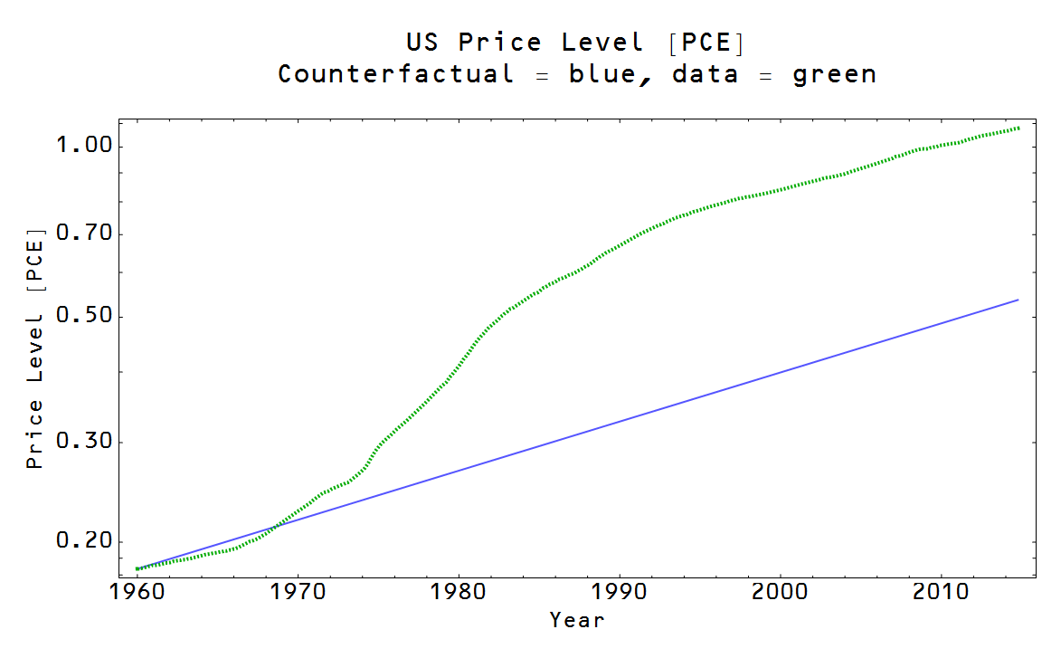
What if US inflation had been 2% since the 1960s?

I am re-watching the PBS program on macroeconomics (made before the financial crisis of 2008, and told from a somewhat triumphal viewpoint of the Chicago school) now that I have a better grasp on economics ... and even my own model. Anyway, one thing that struck me in the discussion of the 'stagflation' of the 1960s and 70s that everyone said was so terrible is that without it, the US economy would be only a tenth of the size that it is today. 

I made a counterfactual economy -- one with a 2% inflation target from 1960. Here are the results for PCE inflation (exactly 2% inflation), the currency base and NGDP:

One interesting thing apparent in these graphs is that the economy made a turn towards 2% inflation starting in the 1980s (under the Volcker disinflation) -- the green curve moves toward becoming parallel to the blue curve. At the same time NGDP growth (red) takes a turn toward being parallel to the 2% inflation rate counterfactual NGDP (blue).

I had always been curious as to what caused the big kink in the economic growth rate in 1980 (higher before, lower after). It appears to simply be a shift from a policy regime that didn't focus on inflation to one that did.

Is the demand curve shaped by human behavior? How can we tell?

I'm in the process of writing (yet another) simple introduction to the information equilibrium view of supply and demand, but stumbled onto an issue that -- while I may be wrong about it -- really seems to fly in the face of basic economics. I asked myself the question: how would we go about determining the shape of the demand curve -- especially in a way that let's us see human behavior at work?

You might think experiments would help here. However e.g. Vernon Smith's approach assumes utility. If you give your agents utility functions that obey the conditions of the Arrow-Debreu theorem, then an equilibrium must result from just the pure mathematics of it, along with the mechanics of supply and demand -- regardless of human behavior. This is basically just a restatement of the idea that assuming homo economicus (by giving people well-defined utility functions) effectively implies ideal markets.

I started to look at some classroom experiments ... and saw that they don't actually demonstrate what they set out to demonstrate.

Take this experiment [1] for example (it is not unusual). The idea is that students write down a reservation price and the instructor collects the cards and tallies up the number that would buy at a given price (or they all stand up and sit down as the price called out gets too high in this version [2]). As the price goes up, the number of students willing to pay goes down. Makes sense.

But is this measuring a demand curve (i.e. things like diminishing marginal utility)? No. And it is especially clear in [1] if you look at their graph. It's not a demand curve, it's an inverse survival curve for a normal distribution:

That is to say it's a cumulative distribution function of a normal distribution turned on it's side (see the second graph here). What this is measuring is the (normal) distribution of price guesses from the students:

It is especially telling that in experiment [2] above, they leave off the last few students -- i.e. the last piece of the CDF where it stops being linear.

This doesn't have anything to do with human behavior. Why is that? Because I can get the exact same "demand curve" using brainless atoms. The contribution to the pressure from one atom is based on the force it exerts against the container -- the change in momentum as it reflects off the wall. That change in momentum is proportional to its velocity, and in an ideal gas, the atoms follow a Maxwell distribution:

If we asked atoms to sit down as different velocities were called out if the velocity was higher than theirs, we'd get the following "demand curve":

I used this example since both price vs demand and pressure (velocity) vs volume come from the same derivation in the information transfer model and neither require human behavior to explain.

Now you might say that students' knowledge of the average price of M&M's (in the example) shows how human behavior enters the equation; they see the value of other goods and make utility judgments. But! Atoms also seem to 'know' the average velocity of the ideal gas in the analogous experiment -- set by the thermodynamic temperature. The students know the value of a packet of M&M's because it is set by the value of money (perhaps set by an economic temperature) -- something controlled by the central bank in most economic models.

So how do we see a demand curve in a way that incorporates human behavior?

In the MR University video, after using 'Black Friday' as an example (which is actually the experiment discussed above), they move on to describing it in terms of substitution. That is definitely human behavior, right? We decide to buy other things with our money!

Well, actually ... how is that different from the experiment above? When you have an estimate of the price of M&M's and the price goes above that reservation price you are effectively making the statement "I'd rather spend my money on something else" (or "I don't have that much money" in some cases). Something being "too expensive" and opting to save the money for something else are logically equivalent statements.

Now you might say that in the case of atoms when things get "too expensive" (too high a velocity) it's because they "can't afford it" (their velocity is all they have), not because they've decided to keep their "money" (velocity) for something else.

And that would be true ... for a single container with an ideal gas. But multiple markets is like multiple containers (with the same number of atoms**, i.e. students) at different temperatures (i.e. prices). So while 20% of atoms have a velocity of at least 1 in one market, 20% will have a velocity of more or less in another, corresponding to 'money' they'd 'spend' on something else.

So, again, how do we see a demand curve in a way that incorporates human behavior?

I'm probably missing something. There could be other experiments*** that show human behavior shining through. Just because I don't know what they are doesn't mean they don't exist.

There is an ulterior motive here, and it's not just that I think starting with humans as optimizing agents is likely not only intractable, but unnecessary. It's that in writing that simple introduction I mentioned at the top of this post I realized that the information transfer model, in an ideal market, has literally nothing to do with the behavior of the agents. Supply and demand are a property of two quantities that are in information equilibrium ... and the mechanics follow**** from D = κ P S. Hold D constant and as S goes up, P must fall (a demand curve). Hold S constant and as D goes up, P must go up (supply curve).

That's all there is ... and if that's all there is ...

Footnotes:

** We are glossing over the the fact that we have the capability to distinguish different people and e.g. assign a particular price estimate in each market to a particular person -- something we can't really do for identical atoms. However, there is the question of whether the market can see people as distinguishable ... using money makes transactions anonymous.

*** You might think of an experiment where you reduce the supply and watch how the price goes up and take a survey and ask why people decided not to buy something. However 1) the mechanism you are using assumes supply and demand, and 2) since you are reducing the supply, some people will have to buy less regardless of how they feel about it. (Humans are subject to post-hoc rationalizations, so the survey would be suspect, anyway.)

**** You can get different shaped demand curves from this equation -- it's actually just an instantaneous equation and P is a derivative (dD/dS).

This is why sociologists think economists are arrogant

Tyler Cowen cites a study that makes claims about inflation and tolerance of the LGBT community

On the other hand, the data shows that when a society has impressive scores on property rights security and low inflation — two other components of economic freedom indexes — these characteristics are strongly and positively correlated with tolerance of gays. It’s possible that low inflation, and the behavior of a central bank, are stand-ins for the general trustworthiness of a nation’s government and broader institutions, and such trustworthiness helps foster tolerance.

That conclusion kinda depends on low inflation being the result of the actions of institutions, doesn't it? That implies a monetarist view, but even if you allow the word 'institutions' to be more inclusive of e.g. a 'fiscal theory of the price level', that still implies some sort of control by national elites at the point of low inflation.

Countries mired in liquidity traps are on average more tolerant? That makes the question seem even weirder. And for market monetarists, a liquidity trap is a sign of incompetent institutions (namely the central bank).

In the information transfer model, low inflation is generally a result of a monetary policy regime being around for a long time. All economies tend toward lower inflation in the long run (see the graph at the top of this post).

That leads us to the conclusion that basically long periods of time with economic stability lead to tolerance.

Which is something well known in sociology.

Simon Wren-Lewis has a good piece on economists and sociologists. There was also this from Stephen Williamson. But it's the armchair sociology that derives from economic analyses that is problematic.

Lee Smolin's take on Arrow-Debreu

I've been reading Lee Smolin's (of loop quantum gravity fame) take on Arrow-Debreu equilibrium (mentioned by Tyler Cowen awhile ago), and I was struck by how much we are looking at the economic problem the same way. It's probably just our shared backgrounds in particle physics. His take is a lot more sympathetic to the idea that gauge symmetries and other mathematics may be of use, something I would probably share if the information transfer model didn't seem to point to non-ideal information transfer or spontaneous drops in entropy from time to time [1]. Anyway, I've put together (mostly just for my own notes) a collection of quotes from Smolin's paper with something similar I've said on this blog. I follow the quotes with square brackets that get at the differences between what we are saying.

Let's go ...

Smolin: We are then interested in the simplifications that may happen in limits of large numbers, such as a large number of agents, or of goods. In these limits there may be universality classes that only depend on a few parameters that characterize the behaviors of the human actors that comprise the economy

Me: In reality, there may be a detailed balance that keeps the equilibria in an equivalence class described by e.g. a given NGDP growth rate. But that's the rub! Macroeconomics is the study of the behavior of those equivalence classes, not the instances of them!

[This is basically the same thing -- universality class is a particular kind of equivalence class.]

Smolin: The observables of economics are accounting and other records. One should then try to construct a theory of economics that involves only observables. The importance of this kind of operational principle in physics and other sciences have been paramount. Let’s see what it can do for economics. This restricts attention to what is actually measured by companies, individuals and governments. And it removes from consideration fictional elements that have nothing to do with how real economies work such as fixed spaces of products, fixed production plans, utility functions etc

Me: Game theory is a representation of economic microfoundations; the information transfer framework makes as few assumptions about microfoundations as possible. We are assuming we don't know any game theory. ... The following is a rough sketch, but one way to think about the information transfer model is as an ensemble of games with random payoff matrices (zero-sum and not) with players repeating games, switching between games and possessing some correct and/or potentially incorrect information about the payoff matrix (or its probability distribution). The only "constraint" is that all of the realized payoffs sum up to a macroeconomic observable like NGDP.

[Where Smolin says leave out unobservable things like utility, I say assume you know nothing about them -- in this case a payoff matrix in game theory is essentially a set of contingent utility functions. Expectations also seem unobservable in this sense.]

Smolin: An analogy to physics might be helpful here. Just like there is micro and macro economics, there is micro and macro physics. The former is atomic physics, the latter includes thermodynamics and the description of bulk matter in different phases. Macrophysics mostly deals with matter in equilibrium. The bridge between them is a subject called statistical mechanics, which is a general study of the behavior of large numbers of atoms, both in and out of equilibrium. Indeed, even though there is not a close analogy between the notions of equilibrium in economics and physics, there is clearly a need for a subject that might be called statistical economics. It would be based on a microscopic model of the basic agents and operations or processes that make up an economy and study the behavior of large numbers of them in interaction.

Me: ... assume the principle of indifference: given the macrostate information you know (NGDP, price level, MB, unemployment, etc), assume the system could be in any microstate consistent with that information with equal probability [2]. In Bayesian language, this is the simplest non-informative prior. This way lies statistical mechanics, thermodynamics and information theory.

[This is the same idea.]

Smolin: Furthermore, since equilibria are in general non-unique, there is no mechanism in the theory to explain why one rather than another of these equilibria could be chosen by the market mechanism. All we know about the market mechanism in the theory is that it looks for Pareto efficient states, but if there are many the market mechanism cannot choose among them.

Me: ... imagine a world where fuel was slightly more expensive and cars were slightly less expensive. Depending on the relative price this could still clear the market with the same amount of money being spent in aggregate on cars and fuel. ... However! If there is less fuel and more cars, then there might be fewer ways to associate gallons of fuel with cars (lower entropy since the fuel is fungible) and you could select the actual equilibrium based on maximum entropy production.

[Maximum entropy selects which Arrow-Debreu equilibrium; this quote represents a possible solution the problem in the quote from Smolin.]

Smolin: Time must be incorporated in a way that recognizes the irreversibility of most actions taken, as well as the asymmetry of the present, past and future.

Me: Basically, because the market is made of people, we can violate the second law of thermodynamics (ΔS > 0) by coordinating ourselves in a way that atoms or particles can't. There is no second law of econo-dynamics because of human behavior -- which is unfortunate because otherwise (if human nature didn't matter) ΔS > 0 would imply ΔNGDP > 0 -- the economy would always grow (absent real shocks like natural disasters or resources running out).

[The second law holds most of the time as there is usually economic growth; a recession represents moving backwards. My arrow of time in economics is essentially the thermodynamic arrow of time, with some exceptions during recessions. Entropy producing processes are irreversible processes. This is another case where what I am saying is a solution to a problem stated by Smolin.]

Smolin: Markets with large numbers of agents have very large approximate symmetries, expressing the fact that there are many individuals with similar educations, interests or aspirations and many firms competing to offer similar products and services. In the steady states reached by real economies these symmetries are usually broken. This leads to multiple equilibria or steady states. The representation theory of the broken symmetries is then relevant to the distribution of equilibria.

Me: If your macro system appears to be described by n << N degrees of freedom, then it seems highly likely that among the total number of microstates, large subsets of the microstates are going to be described by a given macro state -- i.e. the equilibrium (the microstate satisfying macro constraints) is not going to be unique. For example, in an ideal gas, you can reverse the direction of the particle velocities and obtain another equilibrium (actually, all spatial, rotational and time-reversal symmetries lead you to other equilibria).

[There is a slight difference here in that Smolin is being much more accurate from the physics perspective. Equilibria related to each other by a symmetry transformation are not actually distinct (e.g. reversing the particle velocities) in physics. The sense here is that you could exchange iPads for Nexus tablets in theory, but the actual dominance of iPads breaks the symmetry leading to two equilibria: one where the Nexus dominates and one where the iPad dominates.]

Footnotes:

[1] Smolin writes: ... we want to know far from ideal a real economy may be, and still count as evidence for the theory. For example, lets take the prediction that all markets clear in equilibrium. There are clearly lots of markets in the real world that do not perfectly clear. In the information transfer model, we have a theory that tells us the 'neoclassical' view holds if the system is in information equilibrium (we don't have episodes of non-ideal information transfer). Essentially, if the information transfer model holds assuming ideal information transfer, we have evidence for the ideal neoclassical theory -- except for the emergent aspects of macro like liquidity traps and nominal rigidity.

How do you measure the price level?

econ: PCE or CPI? Core or headline?

info: [Sigh] ...

econ: What?

info: They're barely different from each other!

econ: Isn't there a joke about a physicist and a spherical chicken?

That's from me a few days ago. I've been on an anti-utility kick lately and the process, I've been looking at a bunch of stuff on preferences, total orderings and ... differential geometry. Smolin's paper mentioned Malaney and Weinstein's gauge theory approach to price indices. I plan doing a bit more thinking about what Smolin says -- he thinks a non-equilibrium statistical mechanics approach to economics may be useful (like the one I am advocating on this blog), saying: Nonetheless, once one gets past this confusion [about thermodynamic equilibrium], there is still a cogent claim that non-equilibrium statistical mechanics may be a basis for a model of an economy. But for now, I'm going to concentrate on the gauge theory approach to the so-called index number problem.

I seriously dislike the name, because it makes me think of some kind of deep problem in number theory or the Atiyah-Singer index theorem. Oh, well. I don't have much of a choice there. Let's start with Wikipedia:

The "index number problem" refers to the difficulty of constructing a valid index when both price and quantity change over time. For instance, in the construction of price indices for inflation, the nature of goods in the economy changes over time as well as their prices.

Wikipedia continues: "There is no theoretically ideal solution to this problem."

In fact there may be, based on Malaney and Weinstein's differential geometry approach. In her thesis, she motivates an 'economic derivative' that is a covariant derivative. You may remember that this gauge theory approach was part of Chris House's rant about physicists in economics. I opined on this blog, and asked the question that should be asked of any mathematical approach to a problem: what is it good for?

Well, Malaney's approach allows you a way to solve the index number problem ... assuming you buy into the other assumptions. The idea is that a salary $S(t)$ that is always proportional to the 'correct' price index $P(t)$ (with constant of proportionality $\alpha$) should have the same purchasing power, which allows the construction of a covariant derivative

$$
\frac{D}{Dt} = \frac{d}{dt} - \frac{d}{dt} \log P 
$$

So that

$$
\frac{D}{Dt}S = \frac{D}{Dt} \alpha P = 0
$$

This choice what you mean by 'constant' (i.e. derivative equal to zero) solves the index problem, because it essentially makes all of the price indices equivalent to a so-called Divisia index. Don't let the Divisa terminology worry you. Essentially, various chained indices or indices with changing baskets of goods are approximations to a Divisia price index.

The problem economic theorists would have with this is that a Divisia price index is path dependent brought about by changing preferences. Basically, what makes the Divisia price index problematic is the issue of mapping it to utility in the sense that John Kay discusses here.

Would you rather be the richest person in history or live in a time of antibiotics? Divisia answers with the former if you equate the 'inflation adjusted' value of goods with utility as defined in ethical philosophy. The path dependence is obvious here -- because Rothschild would likely value antibiotics today. Malaney argues that this path dependence may be a desireable property in her thesis, but overall, the question of how money equates to utility will probably always be a philosophical one.

As an aside, Noah Smith talks about unstable preferences here. However, the mapping of money and price indices to information lacks these philosophical issues. I've talked about this before -- inflation is better understood as an information theoretical construct rather than a utilitarian philosophical one.

The new bit here is that I want to show that the Divisia price index is the proper measure in the information transfer model, just like in the differential geometry approach of Malaney and Weinstein. The underlying assumption is different, though. In our case, a price index isn't measuring 'constancy' (in Malaney's thesis), but rather 'meaningful aggregation'.

The question we ask is whether there exists a consistent price level $P$ that allows us to treat the economy as aggregate supply $Q$ and aggregate demand $N$ when $P$ is made up of individual prices $p_{i}$ (and likewise $q_{i}$ and $n_{i}$).

If we start with (taking $\kappa = 1$ WOLOG)

$$
N = Q P
$$

Then taking the logarithmic time derivative (this gives a percentage rate when multiplied by 100), we get

$$
\frac{d}{dt} \log QP = \frac{d}{dt} \log Q + \frac{d}{dt} \log P
$$

$$
= \frac{1}{Q}\frac{dQ}{dt} + \frac{1}{P}\frac{dP}{dt} \;\;\;\text{ (1)}
$$

However, if we take the individual markets (I'll use vector notation to simplify the equation a bit)

$$
q \cdot p \equiv \sum_{i} q_{i} p_{i}
$$

$$
\frac{d}{dt} \log q \cdot p = \frac{1}{q \cdot p} \frac{d}{dt} q \cdot p
$$

$$
\frac{d}{dt} \log q \cdot p = \frac{1}{q \cdot p}  \left( \frac{dq}{dt} \cdot p + q \cdot \frac{dp}{dt}\right)
$$

$$
\frac{d}{dt} \log q \cdot p = \frac{1}{q \cdot p} \sum_{i}  \left( \frac{dq_{i}}{dt} p_{i} + q_{i} \frac{dp_{i}}{dt} \right) \;\;\;\text{ (2)}
$$

The Divisa price index $P$ is defined by separately equating the two terms of (1) and (2) and solving the differential equations:

$$
\frac{1}{Q}\frac{dQ}{dt} = \frac{1}{q \cdot p} \sum_{i}  \frac{dq_{i}}{dt} p_{i}
$$

$$
\frac{1}{P}\frac{dP}{dt} = \frac{1}{q \cdot p} \sum_{i}  q_{i} \frac{dp_{i}}{dt}
$$

In the information transfer model, that means $P$ allows you convert between informationally equivalent baskets of goods. That is to say that a basket from 2014 that includes an iPad and one from 1980 that does not can potentially be equivalent in information.

However, an intervening redefinition of money or a monetary regime change will break the direct equivalence between $P$ for different times. That is to say Rothschild's and Kay's utility cannot be compared because they lived in different monetary regimes (a gold standard and fiat currency regime), even if both used 'pounds sterling'.

Interestingly, non-ideal information transfer where $N \geq Q P$ does not affect this derivation -- we are equating the RHS of equations when we equate (1) and (2); both are on the same side of that inequality.

Anyway, more on the Smolin article to come.

Update:

I kind of glossed over the role of the changing information transfer (IT) index (κ) in the more accurate model of the price level in terms of the money supply. In this post, we used an aggregate supply (Q) rather than the money supply (M), so I don't think there should be a time changing IT index in that case. In a sense, PQ = N represents both the expenditure method and income method of calculating NGDP which should be equal (and should have κ = 1).