Nominal rigidity is an entropic force

Commenter pjz brings up transaction costs as a source of nominal rigidity on this post from a couple months ago. In responding, I found a great old post by Mark Thoma about some issues with macro modeling of nominal rigidity.

Basically there are two major mainstream micro approaches to achieve macro nominal rigidity that have observational consequences:

• Transaction (menu) costs: there is a cost to change the price. Price changes should be observed to infrequent and biased towards large changes (frequent small changes would be penalized).
• Calvo pricing: only a sample of firms can change their prices in any one period. Price changes would be observed to be infrequent.

What does the data show? [Pictures from Thoma's post]

Oh ...

Nothing seems to be stopping those prices from changing. Essentially among the 60,000 prices observed, prices are sticky in aggregate but not individually. The two mainstream approaches above imply that prices are sticky both individually and in aggregate, something that is flatly contradicted by data.

How do you get sticky aggregate prices with flexible individual prices? Well, one way is entropy as I show in the post from a couple of months ago linked above. The picture in your head should be much like this one (it shows something different, but the concept is the same):

... thousands of prices fluctuating wildly, with the aggregate level barely moving.

One consequence of this would be that there is no microeconomic explanation of nominal rigidity ... flying in the face of the microfoundations approach to the Lucas critique.

Predicting unpredictability

Paul Krugman, an economist who actually does understand special relativity [pdf], points us to an old post by David Levine:

I feel a little like a physicist at the cocktail party being assured that everything is relative. That isn't what the theory of relativity says: it says that velocity is relative. Acceleration is most definitely not. So were you to come forward with the puzzling discovery that acceleration is not relative...

I don't quite get why economists think the experience of physicists is more relatable than e.g. their own. Let me think of a way to make my point to the readers of Huffington Post using an example they'd be more familiar with ... how about ... a physicist.

Anyway, the principle of relativity is actually a more general principle that the laws of physics are unchanged if observed in reference frames that have a relative velocity to one another. So strike one.

I also think Levine is using the English phrase "X is relative" in the philosophical sense of e.g. moral relativism. X is wrong (or big or small, etc) only relative to something else; there is not some absolute scale by which to measure X. Special relativity actually says the exact opposite: all velocities can be compared with the speed of light and are less than or equal to it. Velocity isn't relative, it is absolute -- compared with the speed of light. So there's strike two.

Brad Delong points out the flaw that accelerated frames are incorporated in general relativity. That would be strike three.

However, let me take a somewhat more charitable view of Levine's statement in order to get at something deeper. He is using it as an analogy for rational expectations -- and instead someone is coming forward and saying that the inability to predict financial crises disproves the EMH. Levine is saying unpredictability is actually a prediction of the theory.

Rational expectations and the EMH aren't being used as intellectual constructs to arrive at the truth here. They are being deployed in a manner similar to creationist "intelligent design". In that case, complicated systems are put forward for which there is no theory as to how they evolved as proof that evolution isn't real. A flagellum is so complicated [1], there is no way it could have evolved!

One's personal failure of imagination is never evidence for or against any theory.

The fact that mainstream economics can't predict financial crises isn't evidence for the EMH. We don't know the fundamental theory of economics yet. Maybe you can predict financial crises. We don't know.

In quantum mechanics, outcomes of measurements are random. That observation is not the evidence for quantum mechanics. The evidence for quantum mechanics are the precise predictions for things that are not random ... and that success is the reason we accept the randomness in quantum mechanics.

Footnotes:

[1] This example is particularly funny because there is a pretty convincing evolutionary pathway for a flagellum.

There is no theory?

I think I mis-categorized Scott Sumner's viewpoint in my posts on expectations here [1] and here [2]. In this post, Sumner says:

The markets view QE as expansionary. The market monetarist view is the market view. Whenever the market changes its view and becomes more Keynesian, or MMTist, or Austrian, or more new classical, I’ll change as well.

In [1], this is actually option 3 (instead of option 4): 

"This implies that all you need to do is convince markets that Keynesianism is right to make Keynesianism right. Or you could convince markets that monetarism is right, which would make monetarism right."

In [2] this is the first of the two possibilities (instead of the second): 

"First, is that E(x) ≈ T[E(x)] doesn't specify T. In that case ... T ... depends on what humans believe and there is no specific theory of pure expectations (or you just have to convince the market that T = X and it is entirely political ... X could be communism or mercantilism or the Flying Spaghetti Monster). "

This is actually remarkably nihilistic (and basically why I misunderstood Sumner's view). Sumner, an economist, seems to believe there is no fundamental theory of economics. The economy of an alien civilization would most likely work entirely differently from ours.

However, I don't actually believe Sumner has ridden this trolley all the way to the end. It means you can't actually use "economics" to explain why one economic theory failed or another succeeded, e.g. as is frequently done in reference to communism. The reason communism failed in this view is because the economic agents didn't expect it to succeed. Likewise, welfare-state economy works fine if everyone expects it to.

Then why does he tout Reagan and Thatcher? According to Sumner's view, their accomplishment appears to be that they introduced confidence and groupthink to the US and UK. Calling this supply-side reforms is then a misnomer. They have nothing to do with "reform" or the mechanics of supply and demand -- remember, there are no mechanics!

What I really think is happening is something like the two-step of terrific triviality. The strong claim is market monetarism is the optimal theory of expectations. The weak claim is that any theory of expectations is possible.

The strong claim is behind Sumner's view of Reagan and Thatcher -- it matters which theory of expectations is the one to rule them all. The weak claim is behind Sumner's reasons to discount other possible explanations -- sure, your mechanism is plausible (or even observed), but what does the market think? In one case, market monetarism is purely an idea. In the other, it is purely observational.

Utility in an information equilibrium model

I've said many times on this blog that the concept of utility is unnecessary (except to solve an information problem); in this post I'll allow utility, but show that even then utility maximization is unnecessary to select an economic equilibrium.  Essentially, I will derive the utility approach to economics using the information transfer model.

Let's define utility $U(x_{1}, x_{2}, ...)$ to be the information source in the markets

$$
MU_{x_{i}} : U \rightarrow x_{i}
$$

for $i = 1 ... D$ where $MU_{x_{i}}$ is the marginal utility (a detector) for the good $x_{i}$ (information destination). We can immediately write down the main information transfer model equation:

$$
MU_{x_{i}} = \frac{\partial U}{\partial x_{i}} = k_{i} \; \frac{U}{x_{i}}
$$

Solving the differential equations, our utility function $U(x_{1}, x_{2}, ...)$ is

$$
U(x_{1}, x_{2}, ...) = a \prod_{i} \left( \frac{x_{i}}{c_{i}} \right)^{k_{i}}
$$

which is a Cobb-Douglas utility function ($a$ and the $c_{i}$ are constant). In the traditional economic approach, the next step is to look at the level curves of this utility function alongside the budget constraint (in a two-good market i.e. two dimensions):

$$
\text{(1) }\; M \geq \sum_{i} p_{i} x_{i} = p_{1} x_{1} + p_{2} x_{2}
$$

The level curve that is tangent to the budget constraint gives us the maximized utility. We show this in the next graph (level curve is the dashed gray curve and the maximized utility point is gray as well):

The entropy maximizing solution is given as the blue dot at the centroid of the blue triangle with the solid utility level curve passing through it. If we take every point that satisfies the budget constraint (1) as equally likely (the blue shaded region), the expected equilibrium value is given by the centroid. Now this centroid moves in effectively the same way as the utility maximum, just at a lower utility value:

The red line shows that at a higher price of $x_{1}$ with the same budget constraint, less of $x_{1}$ can be afforded. Both the utility maxima (gray dots) and the entropy maxima (blue and red dots) move inward towards smaller $x_{1}$ and lower utility, tracing out a demand curve. For two goods, there is only one big difference in the utility maximizing and entropy maximizing models of supply and demand: the entropy maximizing equilibrium doesn't fully saturate the budget constraint.

One possibility is to make the artificial restriction that all income $M$ must be spent. The centroid of the boundary of the blue triangle would essentially be the middle point of the budget constraint line. However, we don't actually have to do this.

If we randomly sample the triangle bounded by the budget constraint, we end up with something like this in two dimensions:

The distribution of the sum $p_{1} x_{1} + p_{2} x_{2}$ is somewhat uniformly distributed between 0 and the budget constraint as shown by the blue line in the next graph:

However, if we increase the number of dimensions (the number of goods in the economy), most of the points are near the budget constraint (the red and green lines). This is a general property of higher dimensional shapes: nearly all of the points are in a thin shell near the surface. That means for a large number of dimensions, the expected equilibrium should be near the budget constraint even without making the artificial restriction above:

Now this point only maximizes utility if every good is in a sense the same -- the budget constraint (1) and the utility function $U$ is symmetric under interchange of $x_{i} \leftrightarrow x_{j}$. Typically, the entropy maximizing point is near the utility maximizing point if neither the utility function nor the budget constraint are wildly asymmetric ($k_{i} \gg k_{j}$ or $p_{i} \gg p_{j}$).

We can't directly observe utility, though. Therefore it is always possible to perform a preference-preserving transformation $f(x_{i}, \alpha_{i}) : x_{i} \rightarrow \exp \alpha_{i} \log x_{i}$ that makes the utility level surface tangent at the maximum entropy point near the budget constraint (or makes the utility function symmetric). [Correction, per LAL in comments below.]

Aside: This framework would allow us to experimentally determine whether utility maximization or entropy maximization represented a better model of microeconomics. Using multiple goods, aggregate the different allocations chosen by individual subjects (every student in a classroom is given $n$ tokens to allocate among $m$ different goods like candy bars or bacon).

Second aside: The typical economics approach appears to be setting $MU_{x_{i}} = \beta p_{i}$; we could accommodate that with an additional information equilibrium condition $MU_{x_{i}} \sim p_{i}$ which would allow $\log MU \simeq k \log p$. The typical approach assumes $k = 1$.

Japan inflation update

The Q4 GDP number is available for Japan so here are the model updates including the new monetary and price level data. I've adjusted the Japanese core CPI for the VAT tax increases [1] in 1997 and 2014.

The prediction for Japan uses the same procedure as for the US predictions (see e.g. here), however I've integrated the inflation prediction errors to generate an error band for the price level (hence the size of the error will grow over time).

Here is the full (un-smoothed) model:

Here is the smoothed result:

And here is the prediction using the smoothed result:

Basically this prediction says inflation will be approximately zero for the next 10 years, barring any re-definition of the Yen.

Footnotes:

[1] Here are the unadjusted versions:

Real vs nominal

I mentioned this in an update to a post from a few months ago on the Solow growth model, but one thing I've noticed in the information transfer model is that adjusting for inflation tends to make the models not work as well. That is to say the models work really well for nominal quantities, but fail for real quantities.

Why is this?

Short answer is: I don't know.

However, I have some ideas that I'd like to discuss in the original spirit of this blog -- thinking out loud. The picture that is forming in my head is that the economy functions based on nominal values -- nominal dollars are the "fundamental particles" of macroeconomics -- while real dollars are more relevant to welfare economics. [1]

This would make sense of money illusion: when humans interface with the economy, they logically do so with nominal values. Humans aren't foolish for not thinking in terms of "real" quantities.

A loaf of bread might cost a few dollars today as opposed to less than a dollar many years ago. It makes a lot of sense to say that our subjective experience (i.e. derived utility) of the same loaf of bread would be the same regardless of how much it costs or when we experience it [2]. That's one way to arrive at the intuition behind real vs nominal values.

Since we ignore utility maximizing behavior in the information transfer model, we don't need the real value of a quantity to build a causal relationship with another quantity. In the Solow growth model linked above we don't need to relate real capital to real output. Nominal dollars are the fundamental particles, so we look at nominal output and nominal capital (along with the "nominal" labor force).

The information theory at the heart of the information transfer model is mostly about counting the arrangements of objects -- naturally the objects at any given time would seem to be nominal objects.

But!

The information transfer model still has something called "inflation" in it. What is it doing if not adjusting for those relative costs of a loaf of bread above? Well, it is counting the greater and greater amount of information that has to flow back and forth to keep two growing distributions in information equilibrium [3].

Two distributions being kept in approximate information equilibrium per this post.

This view is similar to my rather odd speculative view of why economists are paid more than sociologists in a footnote here. Things in general get more expensive over time because there are more ways to choose a particular basket of goods from a larger economy with more and more varied goods. It takes more information to specify a loaf of bread to be in your basket, so its nominal cost is greater relative to its nominal cost from many years ago [4]. 

Note that the price level is directly related to how much the economy would expand if it found itself in a state with a larger money supply in the absence of shocks or frictions. I called this measure ideal NGDP. That means the price level is more directly measuring this abstract counting argument for the price of all goods. However there is some information loss and the nominal economy does not register this full increase in the "value" of goods -- measured NGDP is lower than ideal NGDP.

When you divide measured NGDP by the price level, you are dividing the realized value of all goods and services by the ideal price. That would essentially represent the realized growth of the economy without the growth in the combinatorial factors. If you think human experience of value/utility shouldn't be affected by simple combinatorial factors (just because there is more stuff around, it doesn't mean we should experience it differently), then this may well be a useful concept.

Footnotes:

[1] In physics, there is usually a difference between the fundamental particle content of a quantum field theory and the effective particle content of a theory. For example, quantum chromodynamics operates on quarks and gluons (the fundamental content), but at low energies you never see either, only baryons and mesons. However, one interesting thing is that when you look at mass or charge renormalization for an electron in quantum electrodynamics, you can make a pretty good theory from ignoring the loop diagrams and just using the experimentally observed values of the mass and charge in the tree level theory.

[2] However people enjoy wine more when they think it costs more, and bread is probably tastier when you're hungry than when you're not. But ignore these complications for right now.

[3] This is from an answer to a question on this post:

The additional information comes from the increased number of bits required to describe the allocation of an increased number of goods sold/demanded. If there are 3 widgets and two agents, there are 4 ways to allocate the widgets (3 + 0, 2 + 1, 1 + 2 and 0 + 3). If there are 4 widgets and 2 agents, there are 5 ways. That's an increase in the information content of an allocation of about 1/3 of a bit: log_2(5) - log_2(4) = 0.32.

[4] Certain rarer goods reveal a lot more information when they are discovered in your basket (think here of flipping a fair coin vs rolling a fair 20-sided die), so they are more expensive. This wouldn't be the only mechanism at work, but I think this argument represents the information equilibrium answer to the paradox of value. Why are diamonds so much more valuable than water when we need water to survive, grow food, etc? The 19th century solution (that is still with us) was marginal utility. Information equilibrium says that diamonds are more valuable because if they appear in a basket of goods, they reveal a lot more information than a gallon of water. I should probably do a whole post on this.

Note that this may be the same explanation behind the values of Scrabble tiles. The Q's and Z's are the diamonds of Scrabble tiles -- they more strongly specify which words in the English language you can spell than the A's and E's (or blank tiles).

Price level model code

One other thing that came out of my interaction with econjobrumors forum is that I should release the code I use (I had previously just put an email contact on the sidebar for requests for the code). There really isn't that much to it. I fit a function to some smoothed data. The majority of the real programming is actually the LOESS filter.

Here is a link to a PDF of the price level model code itself (runs in Mathematica 8). [I hope this works -- I've never used a public link to my Google Drive before.]

Here is what passes for the documentation:

The first two parameters indicate the smoothing done with the LOESS filter, and the next piece of the code is the filter itself.

The next few lines import the xls files that were exported from FRED (I cut out my username from the file paths). In particular, for the monetary base, I use the full base and subtracted out the reserves. I show what the smoothing does to the monetary base data. Additionally I use the convention that a given measurement comes at the end of the measurement period: monthly base numbers come from the end of the the month ... effectively the beginning of the next month (all approximately equal in length). The same with quarterly data. I plan on dealing with the minor issues introduced by this at some point, but really neither the accuracy of the data nor the accuracy of the model calls for it.

The FRED links:

AMBSL
RESBALNS
GDP
PCEPILFE

The next piece sets the limits for the data to be used, and after that is the curve fitting that is solved as a minimization problem. You can see an error that pops up because minyear = 1959. and the first data point is actually from January 1959, or 1959 + 1/12 ~ 1959.08.

The next piece plots the function with the fitted parameters and then I generate a set of points for inflation by taking the instantaneous derivative of the log (the is the continuously compounded annual rate of change). Then I plot the inflation points.

You may see that the curve looks a little different on some of the posts. That's because 1) there is a little bit of sensitivity to the initial point of the minimization and 2) there is another version that fits to the inflation points instead of the price level points, only using the price level fit to fix the constant ΔUS. I'll put that code up too.

Send. More. Parameters.

Noah Smith, on Monday:

Modern macroeconomics is chock full of [dynamic] models. There are as many of them as there are grains of sand on a beach. You can have your pick, since macroeconomic data is typically too weak and uninformative to rule in favor of one or the other. Furthermore, each of these models has a number of parameters that represent how the economy responds to things. The range of parameter values used in models is enormous, since no one knows what the right model is in the first place.

Of course these uninformativeness of the data is directly related to the number of parameters used. The more parameters, the more uninformative the data will be. If the Standard Model of physics had 200 parameters instead of 20 or so, the data would have ruled out fewer competing models and physics would be in the same situation.

So the idea of whether macroeconomic data is powerful or not is dependent on how many parameters you think a macroeconomic model should have. Noah apparently thinks they should have a lot.

The price system as a communication channel

I may have gotten into an argument with an anonymous commenter on the Economics Job Market Rumors forum whose entire argument seems to be on the order of "info theory is wrong LOL". Sometimes even this kind of arguing can be useful, though; it makes you look at the big picture.

See, the thing is, even if the information equilibrium model is not useful for economics, economists must have some view of the price mechanism as a communication channel. If there is information flowing in markets it has to originate somewhere, move through a channel and finally end up somewhere.

I tried to think of what that communication channel could be -- maybe this is wrong (LOL), but it's a start. So let's start with Shannon's A Mathematical Theory of Communication and his famous diagram:

Fig. 1: A communication channel.

What we have is an information source on the left that is encoded and transmitted through a channel (where some noise can be added), to be received and decoded at the destination on the right side. A faithful reconstruction on the right side essentially requires getting the distribution of possible messages on the left side to equal the distribution of possible messages on the right side. For example, at a bare minimum, the distribution of letters in English words must be equal on both sides of the channel for communication (information transfer) to occur. In that case the transmitted information is equal to the received information, or I(Tx) = I(Rx).

In economics, the typical description of the price mechanism is as an information aggregator. All of the many details of e.g. weather patterns, the governments that have dominion over the available arable land, seed genetics and crop yields are compressed into a single number and its movements, e.g. the price of wheat. Agents buying and selling wheat are the source of information that is transmitted by the market and received by the market price.

Fig. 2: Modern economic view of the market as a communication channel.

Even if we had a multidimensional normal distribution (made up of independent distributions) on one side and a normal distribution of price movements (all with the same variance V) on the other we'd still have

(k/2) log 2 π e V - (1/2) log 2 π e V = ((k-1)/2) log 2 π e V

of information loss. A more concrete example: imagine the set of outcomes you can get from rolling 5 dice and trying to encode those outcomes with the set of outcomes you can get from rolling a single die -- you basically lose 4 dice of information.

In this picture, I(Tx) >> I(Rx), which is effectively the view of Stiglitz (2000) [1]

"The exchange process is intertwined with the process of selection over hidden characteristics and the process of providing incentives for hidden behaviors."

The realized real-world distribution over those characteristics and behaviors is the "complex multidimensional distribution" in the diagram above. The lost four dice of information in the example are these "hidden characteristics". Basically, you lose something going from the distribution on the left side to the single-dimensional distribution of price movements on the right side.

Economics had been working with a rather good solution to this problem for the previous 200 or so years: utility. Instead of a complex multidimensional distribution on the left side, economic agents have a single-dimensional distribution of utility for e.g. wheat. When the price of wheat is high relative to a given agent's utility, the agent doesn't buy it. We replace the previous diagram with this one:

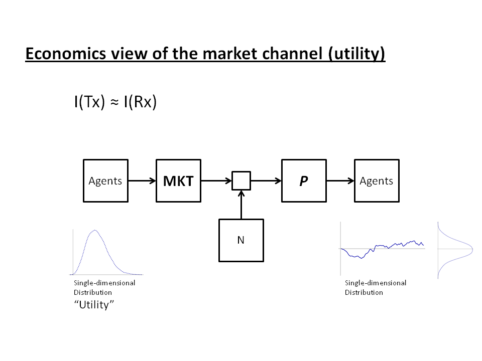
Fig. 3: Utility view of the market as a communication channel

and the information on the right side is approximately equal to the left side: I(Tx) ≈ I(Rx).

[Note that this diagram is an information transfer model and effectively says that utility of a good is in information equilibrium with the price of that good.]

Of course, markets aren't perfect and this description doesn't empirically match up with what happens in the real world (the impetus for the work of Stiglitz to show that the real picture is more like Figure 2). Let's look at the information equilibrium diagram:

Fig. 4: Information equilibrium view of the market as a communication channel.

How does the information equilibrium view differ from Figures 2 and 3? First, we have complex multidimensional distributions on both sides. Supplies and demand for wheat is different in different locations around the world. Different countries use different amounts of wheat (in some places e.g. rice is the dominant carbohydrate source), and different uses of wheat are more valuable than others (ethanol, bread). Wheat is subsidized in some countries (and states within those countries). Some people aren't able to afford as much as others. In a functioning price system, the spatial and temporal distribution of demands for wheat is equal to the distribution of supplies of wheat. There is a loaf of bread for you to buy at the price you want at the store in your neighborhood.

Second, we've moved the price from being the receiver (aggregator) of information to simply being a detector of information flow. Prices are high when small changes in the distribution on the right cause (or are caused by) large changes in the distribution on the left. Prices are low when large changes in the distribution on the right cause (or are caused by) small changes in the distribution on the left. When the distributions change the same amount, we say the price is in equilibrium [2]. The price is still not a perfect detector of information, but over time as the distributions on the left and right evolve, the price will reach an equilibrium.

In this picture I(Tx) ≈ I(Rx) for an ideal market. However, all we can really guarantee is that I(Tx) ≥ I(Rx), so there may well be times when the market isn't ideal and I(Tx) > I(Rx).

Just because it is different, doesn't mean it is right. And if it is right, that doesn't mean it is useful. Maybe in the real world I(Tx) >> I(Rx) most of the time. However, economists must have some picture in their head of the price system as a communication channel if it moves information around, and you can't violate mathematical theorems.

Otherwise ... econ is wrong LOL.



Update 3/23/2015

In looking again at the utility solution, there is still a massive loss in information going from preferences to utility. Well-behaved preferences (essentially ensuring transitivity so that preferences represent a well-ordered set and therefore roughly equivalent to a real-number representation like utility) wouldn't have as much of an issue, but are empirically false.

The mathematical space of preferences cannot be mapped one-to-one to the manifold of utility -- many different sets of preferences will map to the same utility.

What we have is a water balloon of information. If we try to squeeze it down into utility, it bulges out on another side.

Footnotes:

[1] "THE CONTRIBUTIONS OF THE ECONOMICS OF INFORMATION TO TWENTIETH CENTURY ECONOMICS" JOSEPH E. STIGLITZ (2000). (H/T to afinetheorem for linking to it recently.)

[2] One can measure the information difference between two distributions with the Kullback-Liebler divergence. When one distribution changes, that represents a change in information. That information flows through the market an is registered as the commensurate change in the other distribution.

Undershooting inflation

Scott Sumner has a post up today that references a prediction market's estimate of inflation over the next five years (from a NYT article by Justin Wolfers). The prediction market is telling us the Fed will undershoot its inflation target. I commented on Sumner's post, but here is the information transfer model's prediction of the same thing. The latest update for the prediction itself is here. I generated 1000 random paths (using both a Gaussian and empirically derived probability distribution [1] for the errors), and integrated them over the next 5 years to produce a 5-year inflation prediction [2].

Here are the first 200 of those 1000 random paths:

And here is the resulting prediction using roughly the same graph as the NYT article (which I adjusted using Sumner's PCE inflation correction of -0.35% [3]):

Here it is with higher resolution for the IT model prediction:

Footnotes:

[1] The empirical distribution didn't come up with a very different result, so I am only showing the normal distribution results.

[2] Note that the 5-year prediction is right in the sweet spot of the IT model's capability.

[3] The prediction market used CPI inflation, so I adjusted the distribution to show PCE inflation by fitting an empirical distribution to the CPI prediction market data and shifting that distribution by 0.35%, per Scott Sumner's adjustment in his post linked at the top of this post.