The Euler equation as a maximum entropy condition

In the discussion of the RCK model on these two posts I realized the Euler equation could be written as a maximum entropy condition. It's actually a fairly trivial application of the entropy maximizing version of the asset pricing equation:

$$
p_{i} = \frac{\alpha_{i}}{\alpha_{j}} \frac{\partial U/\partial c_{j}}{\partial U/\partial c_{i}} p_{j}
$$

To get to the typical macroeconomic Euler equation, define $\alpha_{i}/\alpha_{j} \equiv \beta$ and re-arrange:

$$
\frac{\partial U}{\partial c_{i}} = \beta \; \frac{p_{j}}{p_{i}} \; \frac{\partial U}{\partial c_{j}}
$$

The price at time $t_{j}$ divided by the price at time $t_{i}$ is just (one plus) the interest rate $R$ (for the time $t_{j} - t_{i}$), so:

$$
\frac{\partial U}{\partial c_{i}} = \beta (1 + R) \; \frac{\partial U}{\partial c_{j}}
$$

And we're done.

The intuition behind the traditional economic Euler equation is (borrowed from these lecture notes [pdf])

The Euler equation essentially says that [an agent] must be indifferent between consuming one more unit today on the one hand and saving that unit and consuming in the future on the other [if utility is maximized].

The intuition for the maximum entropy version is different. It does involve the assumption of a large number of consumption periods (otherwise the intertemporal budget constraint wouldn't be saturated), but that isn't terribly important. The entropy maximum is actually given by (Eq. 4 at the link, re-arranged and using $p_{j}/p_{i} = 1 + R$):

$$
c_{j} = c_{i} (1 + R)
$$

The form of the utility function $U$ allows us to transform it into the equation above, but this is the more fundamental version from the information equilibrium standpoint. This equation says that since you could be anywhere along the blue line between $c_{j}$ maximized and $c_{i}$ maximized on this graph:

the typical location for an economic agent is in the middle of that blue line [1]. Agents themselves might not be indifferent to their location on the blue line (or even the interior of the triangle), but a maximum entropy ensemble of agents is. Another way to put it is that the maximum entropy ensemble doesn't break the underlying symmetry of the system -- the interest rate does. If the interest rate was zero, all consumption periods would be the same and consumption would be equal. A finite interest rate transforms both the coordinate system and the location of maximum entropy point. You'd imagine deforming the n-dimensional simplex so that each axis was scaled by $(1 + r)$ where $r$ is the interest rate between $t_{i}$ and $t_{i + 1}$.

Footnotes:

[1] The graph shown is actually for a large finite dimensional system (a large, but finite number of consumption periods); the true entropy maximum would fall just inside the blue line/intertemporal budget constraint.

The importance of transversality conditions (more on the Ramsey model)

There has been some fun and interesting discussion of the Ramsey-Cass-Koopmans [RCK] model on this post of mine. Sorry to those in the discussion that I haven't gotten back to the comments yet -- I've been taking my time to think about what's been brought up. I noted at the end of my post that:

Now there is some jiggery-pokery in the [RCK] model -- economists include "transversality conditions" that effectively eliminate all other possible paths [in the phase diagram].

This was not some throw-away line in the conclusion; it was the key point of the post. I think LAL's comment is a really useful way to understand how Nick Rowe and I ended up talking past each other:

I think you should pay more attention to the transversality conditions...there is a lot more economic content to them than you are realizing...

I completely agree that there is a lot of economic content! I think this is what Nick Rowe thought I kept missing when he metaphorically threw the eraser at me sitting in the back of the class ("What's the difference between pendulums and people? People have plans and expectations about the future, that affect their current actions."). However, my main point was that the transversality conditions (enforcing those plans and expectations about the future) are practically all of the economic content of the RCK model -- the RCK equations are somewhat superfluous.

Let me start with the explicit numerical model, parameters and all:

This system of differential equations has a "saddle path" solution that runs from from a pair of initial conditions for capital and consumption to the equilibrium point. In the next graph I show the saddle path (black), the (approximate) equilibrium (black point) along with 2000 paths randomly distributed within 1% of the initial conditions that lead to the saddle path:

As you can see, most of these paths diverge from the saddle path -- and that's just for being 1% off. So given measurement error and random events, you are unlikely to find yourself exactly on the saddle path.

One of the main purposes of the transversality conditions is to say nearly all of those 2000 paths don't make economic sense. I borrowed this particular description of the argument/intuition from these lecture notes [pdf], but in general this is what Nick was getting at:

Imagine a path along which consumption is falling and k is therefore growing very large. Along such a path the product u'(c) k would grow rapidly, probably causing the limit [to violate the transversality conditions]. Such a path could not be optimal, however, because the economy is accumulating excessive hoards of capital, the output of which never gets consumed because it is reinvested instead. It would pay for the economic planner to slightly and permanently increase consumption, an option that is perfectly feasible given the rapid growth in k.

What this means in the context of the RCK model is that if the economy finds itself on one of those 2000 paths that aren't the saddle path, the economic agents realize a better deal can be had by reducing capital (or reducing consumption) in order to bring the economy back to the optimal saddle path. The result of that (exaggerated for clarity) is a set of path segments of the RCK model (blue) along with corrections (orange dashed) intended to bring the economy back to the saddle path (black line):

You can think of the blue segments as the times when the economy is obeying the RCK model and the orange loops as the times when the economics enforcing the transversality conditions is driving the economy. And this is where we come to my point: most paths would consist of mostly those loops since nearly all paths in the neighborhood of the saddle path diverge from the equilibrium point.

That is to say the typical path would be incredibly jagged [1]. Most of the time it would not be following the RCK saddle path -- or even obeying the RCK model equations, but instead would be on some correction jog taking the economy back to the saddle solution because of the transversaility conditions [2]. A typical path would look like this:

It would be entirely orange corrections (due to transversality conditions), rather than blue RCK solution paths. An ensemble (or path integral) of such paths would average (integrate) to the RCK saddle solution (which I mentioned in my reply to Nick Rowe). But an ensemble would also do that without the transversality conditions. If we just average all the 2000 paths [3] in the graph at the top of this post, we get the result we want (the saddle path, approximately) without assuming the transversality conditions or the economics they entail:

That means the necessary transversality conditions that end up representing most of the economics of the RCK model if understood in the neoclassical sense (i.e. why only 1 of those 2000 paths turns out to be valid) are actually unnecessary. The RCK model equations (at the top of the post) should be understood as establishing all possible ways to consistently divvy up capital and consumption over time. The transversality conditions say that only one of those ways is valid by fiat. An ensemble approach says that all ways are valid, but observations should be consistent with the most likely path.




Update 6/30/2015

If I understand Nick Rowe's comment below ("If rational, [Robinson Crusoe] would jump [to the Saddle path] immediately, and stay on it forever.") the picture looks more like this:

I agree that is the rational (model-consistent) expectations view, but in that view the transversality conditions do next to nothing. They apply once when Robinson Crusoe is first stranded and calculates how much rum he has. After that, Crusoe lives a 'feet up, mind in neutral' beach bum life -- not having to worry about having drunk too much of the rum or too little. He's no longer an optimizing agent, but passively obeying the differential equations at the top of this post.

There are also the questions of a) how do you know what the saddle path is? and b) how do you determine if you're on it? Robinson Crusoe has to spend a finite amount of time figuring out the path and his location relative to it to a given (finite) accuracy ... something that gets infinitely harder as you approach the equilibrium. And valuable drinking time to boot!

Footnotes:

[1] This is actually what happens in Feynman path integrals -- the set of smooth paths has measure zero, so a typical path contributing to the path integral is a noisy path "near" the classical solution.

Graph borrowed from here.

[2] These corrections would be the inputs to control the inverted triple pendulum in the example Tom Brown mentioned. In that example, the controller spends most of its time making tiny corrections (analogous to the orange paths in the graphs above), not letting the pendulum follow the laws of physics (analogous to the blue paths).

[3] It becomes numerically unstable in the brute force way that I've implemented the model and the actual solution wasn't exact so I was unable to show the whole path on account of an outbreak of laziness in finding the exact solution and making sure the random path initial conditions weren't biased (as they seem to be ... towards the all-consumption solutions).

The Keynesian monetarists

From my post Keynesian economics in three graphs

There seem to be a lot of closet Keynesian monetarists out there. I noticed that a large fraction of the massive deficit reduction in the U.S. from 2012 to 2013 was due to dividends paid by Fannie Mae and Freddie Mac, and the big question that's come out of it is whether it should count as a negative ∆G. That is to say we've apparently figured out it's relevant and now we're just arguing over the multiplier. And now the monetarists are the ones arguing that its multiplier should be large (in order to show that the Keynesian view is wrong, of course, but still).

Now I'm not really an economist; I just play one on the internet. I'm a physicist. But I have constructed an economic framework that allows you to build some basic monetarist and Keynesian models from information theory (the main purpose of this blog). In the most empirically accurate versions of the Keynesian model, all that really matters in a recession are strongly coordinated movements of government output. The negative impacts of tax increases would be diffused. Effectively the multipliers are large for spending and small for taxes, As a result you get the "paleo-Keynesian" finding that even deficit neutral expansions of government spending are expansionary in a recession. But the framework also allows you to construct a monetarist model (it's not as empirically accurate over the past few decades, though [1]), so that puts me right where ... well, where many modern Keynesians are as they believe in monetary policy when outside a liquidity trap and fiscal policy when in one.

The more traditional analysis of multipliers looks at their effect on people's behavior -- in particular current consumption. For example, government spending on a building a bridge employs someone who might not be otherwise employed (in a recession), financing their consumption which is spent at stores who then don't have to cut back the hours of their employees which finances their consumption, and so on. Integrating this effect results in a multiplier greater than 1 ... a bigger bang for your government spending buck.

Tax cuts have less of an impact in most (Keynesian) analyses. They apply to people already with jobs, and since the problem of a recession (in the Keynesian view) is an outbreak of frugality, they tend to get saved. At least if you're already saving money; tax cuts for people living paycheck to paycheck are more likely to get spent.

Roughly the opposite reactions with the same multipliers should occur for government "austerity" (increasing taxes and cutting spending).

So how do we treat the dividend payout from Fannie and Freddie?

Matt Yglesias viewed it at the time as being wasted -- it could have been better paid out as government spending, tax cuts or a "helicopter drop" of cash. And that's true.

Sumner says Matt said the "GSE dividends were a contractionary “disaster.”", but I think Matt's view is better characterized as a comparison between a positive and a zero multiplier use of the dividends -- between high multiplier spending and zero multiplier deficit reduction (he said thw word disaster, but not the word contractionary):

The only problem is that this gusher of federal revenue is actually an economic disaster. ...

... the profits aren’t letting us spend more, they aren’t letting us tax less, and they aren’t freeing up private investment capital either. They’re doing nothing. It’s as if the money were sitting around as cash in a storage locker somewhere.

Some commenters and even Sumner suggest that somehow the dividends should be treated as contractionary with a multiplier greater than zero. 

If we view the dividends as a confiscatory tax on those who would have done something with the money if they had held the stock, the multiplier would be small. It's a progressive tax increase applied to people already "saving" (holding the stock). It is unlikely to have financed current consumption. In that case it would be very slightly contractionary.

It could also be viewed as a tax on people paying their home loans, but unlike income taxes in the U.S. the people paying these taxes are getting something directly (housing) in return. It is not a tax that requires people to cut back their consumption. The contractionary effect would be very small indeed -- approximately zero.

Commenter LAL puts forward the idea that the money is leaving the flow of money around the economy and something like this is probably the best argument that it is contractionary. The effect would come though the "shortage of safe assets" view of a liquidity trap -- the dividends mean that additional US treasury bonds (safe assets) aren't issued. Every treasury bond gets us that much closer to a sufficient stock of safe assets that we exit the liquidity trap so in not issuing bonds we're deeper in the trap than we would be if we had.

However, all of these "it's a tax" views are based on a counterfactual world in which the dividends exist and end up in the hands of the private economy and we're looking at the contractionary effect of the opportunity cost.

My original take in a comment on Sumner's post was that the money could be treated as simply a 20 dollar bill on the sidewalk snatched up by the government. Fannie and Freddie were bankrupt and were bailed out. The money otherwise wouldn't have existed ... not otherwise be financing consumption. In that sense, it almost seems like seigniorage: the money booked by the Treasury when it prints physical currency. Before the currency existed, there was no money. Before the US government took over Fannie and Freddie completely, there was no (actually negative) company value or stream of profits.

As I said I am not an economist, so I'm not sure what the correct treatment should be. I will ask Robert Waldmann, the only Keynesian who'll (potentially) take my questions at this point. From my rudimentary knowledge (and the workings of the information transfer model) it seems that the multiplier should be in the small to zero range.

Overall, there is a strange methodology at work here, though. The monetarist premise seems to be that the Keynesian theory multiplier must be large (m ~ 1) in order for the Keynesian theory to be wrong. That is just odd to me. The evidence is that if the Keynesian theory (K) is correct, the multiplier is small (m ~ 0)

P( m ~ 0 |K) >  P( m ~ 1 |K) ≈ 0

So that the Bayesian view with Keynesian prior is:

P(K | m ~ 0) =  P(m ~ 0 | K) P(K)/P(m ~ 0)

which is greater than zero here. But the monetarist premise contains the factor:

P(m ~ 1 | K) P(K)

where they are trying to show both probabilities are near zero. But P( m ~ 1 |K) is small (approximately zero), so P( m ~ 1 |K) P(K) ≈ 0 even without P(K) ≈ 0.

Basically the result you should get out this analysis is that the multiplier isn't large, not that the Keynesian view is wrong.

Footnotes:

[1] Actually, it can be written as a single model that has two limits: an ISLM-like model and a QTM-like model. The ISLM limit is more accurate today, while the QTM limit was more accurate in the 1970s. At least for the U.S. -- other countries like Russia and China are in the QTM limit, Japan is in the ISLM limit, and Canada is at the transition.

Always look at the data (Keynesian economics edition)

Scott Sumner says that we had a half a trillion dollars in deficit reduction from 2012 to 2013:

At the time, I was under the misapprehension that many Keynesians thought a massive and sudden reduction in the federal budget deficit would constitute “austerity” and hence would slow growth. Now that the dust has settled, we can calmly look at the data: 

Calendar 2012: Budget deficit = $1061 billion 

Calendar 2013: Budget deficit = $561 billion 

A reduction of $500 billion in one year. I used to be under the impression that Keynesians thought this would be a disastrous policy that sharply slowed growth.

It's true! That's a huge amount of deficit reduction all at one time. It's sharply visible on this graph of Federal receipts and expenditures:

It's nearly as big as the ARRA -- almost a 20% rise in Federal receipts. It definitely should give Keynesians pause. Or at least a reason to dig into the data ... I mean how do you get nearly a 20% rise in Federal receipts with the economy essentially giving a collective "meh" ... ? Monetary offset is one way. However, it turns out it is nearly entirely due to a single source: dividends from Fannie Mae and Freddie Mac [pdf from BEA]:

That accounts for over half of the deficit reduction between 2012 and 2013. You can see things in perspective if we subtract this piece from the graph above (the old receipts line in gray now):

The other half primarily comes from (from the BEA [pdf]):

Contributions for government social insurance accelerated as the result of an acceleration in social security contributions that reflected the expiration of the “payroll tax holiday” at the end of 2012 and to a lesser extent, the introduction of a hospital insurance tax surcharge of 0.9 percent for certain taxpayers.

Without those two pieces, there would be effectively zero deficit reduction -- there don't seem to have been any significant spending cuts, only a tax increase. And the tax side has a lower multiplier than the spending side (see e.g. here [pdf]) in the typical Keynesian analysis.

The Keynesian effect of the so-called "austerity" in 2013 would have been relatively small (this is just the deficit reduction divided by NGDP compared with NGDP growth):

It would have been completely lost in the noise.

...

Update:

Sumner responds.

Ramsey model and the unstable equilibrium of a pendulum

Also in Romer's Advanced Macroeconomics is the Ramsey-Cass-Koopmans model (here is Wikipedia's version). It has some of the same flavor as the Solow model, but it has a rather silly (from this physicist's perspective) equilibrium growth path:

We are expected to believe that an economy not only will start out (luckily) somewhere on the path from F to E in the diagram above (you can extend F back towards the origin), but will in fact stay on that (lucky) path until reaching E at which point it will stay there (with a bit of luck).

This is a bit like a believing a damped pendulum, given just the right swing from the just the right height, will go all the way around and just come to a stop so that it is "bob-up" like in this picture from Wikipedia:

My first reaction to seeing that growth phase diagram was to laugh out loud. Economists couldn't be serious ... could they? Now it isn't strictly impossible, but the likelihood is so small that the tiniest air current will cause it to fall back to one of the more normal equilibria:

But the phase diagram from the Ramsey-Cass-Koopmans model is basically equivalent to the phase diagram of a damped pendulum near one of its unstable equilibria:

So basically, according to the Ramsey-Cass-Koopmans model, all economies head towards being all capital or all consumption. Who thought this was a good model?

Now there is some jiggery-pokery in the model -- economists include "transversality conditions" that effectively eliminate all other possible paths. If I eliminate all other paths besides the ones that lead to the unstable equilibria in the pendulum case, I get magic pendulum that stands on its head too!

The quantity theory of money as an ensemble average

Using the partition function approach of this post, I looked at the distribution of inflation rates given a log-normal distribution of monetary base sizes and growth rates. The intent was to figure out this picture from David Romer's Advanced Macroeconomics:

I added the naive quantity theory of money result (inflation = monetary base growth) in blue to the figure above.

For a simple model, it was pretty successful (10000 random economies made up of 1000 random markets). The colors indicate density of those random economies (red = highest). The results mostly fall just below the quantity theory line (in black on this figure) just like the case in the picture from Romer's textbook.

We've essentially reproduced the quantity theory as an ensemble average of random markets, that is to say:

〈i〉= 〈m〉

where i is inflation and m is monetary base (minus reserves) growth (angle brackets mean ensemble average).

For completeness, this followed entirely from the price level calculation in the partition function post linked above. The expected value of the price level of the economies looked like this (showing 100 random economies -- each line -- with 1000 random markets):

Nick Rowe shows us the prior

Fixed this (borrowed) graphic per the comment below.

Nick Rowe has a great post up today that really lays out the prior behind monetarism. He simply holds that the government may be good at providing some things, but progressively worse at providing more and more of the economy.

Why? That's just assumed as the prior before gathering evidence. The government is made of people just like businesses, but when a person works for the government, that person's marginal product is lower for some unexplained reason. My marginal product for the company I work for is X, but my marginal product in a government job is α X with  0 < α < 1 because reasons. Let's just cede that point to Nick. Maybe it's true.

However! Regardless of what my marginal product α X is, it simply must be greater than a position in what Matt Yglesias called the unemployment sector. That is to say α X  > 0 for all reasonable estimates of α.

And fiscal policy directed at companies (via e.g. government contracts to build stuff) to hire at full marginal product X > 0 also is better than people working in the unemployment sector. Therefore fiscal policy should essentially be directly correlated with the unemployment rate. The only way the unemployment sector should be large in a country is if you have simply run out of things to do -- everyone's marginal product is zero.

Nick's argument ignores the existence of a very unproductive sector of the private economy ... the unemployment sector.

Ignoring the flexibility, prices are rigid

I was reading Noah Smith at Bloomberg View:

For example, consider the work of rising stars Emi Nakamura and Jon Steinsson of Columbia University. The dynamic duo of Nakamura and Steinsson set out to investigate the idea that price "stickiness" -- the inability of prices to adjust to changing economic conditions -- is a big factor in causing recessions. The stickier prices are, the more a fall in aggregate demand will damage the economy. Nakamura and Steinsson found that a lot of the non-sticky prices in the economy are concentrated in a few items, such as gasoline, or the result of temporary sales and discounts.

When you account for these price patterns, overall prices in the economy look a lot stickier than economists previously thought.

What does this even mean? Ignoring the flexibility, prices are really rigid? I've written about this before (see here or here), but if a price can do this:

because some executive or the marketing department wants to have a sale, why can't it do that because there is a recession? If I can discount prices by 25-50% on a whim, why can't I discount them for a reason?

Not being able to do that just doesn't make any sense to me. That's why I think prices are micro-flexible, but macro-rigid. But maybe I am misunderstanding something?

Is information transfer economics hard?

The basic premise of information transfer economics: if I shake one end of a jump rope tied to a tree in Morse code, the tree feels a force that can be used to reproduce my input signal. If I shake NGDP in Morse code, hours worked should fluctuate in such a way to get that pattern back out. Image from Wikimedia Commons.

I admit I have trouble understanding what others find so difficult about the information transfer framework for economics. For example, Scott Sumner writes:

But he [meaning me] went even further than the other two [Matt Yglesias and Britmouse], creating a revolutionary new type of economics called “Information Transfer Economics.”  Although I’ve tried to understand his model, it’s all way over my head. He knows a lot more math than I do.

I'm pretty sure Sumner was being sarcastic when he called it 'revolutionary'. However, Sumner actually writes down an information equilibrium [1] model on his blog for what he considers to be his own model. In this post we have an hours worked delta (from a "natural rate") related to an NGDP delta (from a future market or central bank target). The key point to understanding the information equilibrium view is to see fluctuations aggregate demand transmitting a signal to hours worked -- i.e. a wiggle in NGDP shows up as a wiggle in H.

$$
\frac{NGDP - NGDP^{T}}{H - H^{n}} = \frac{\Delta NGDP}{\Delta H} = \alpha ' \frac{NGDP}{H}
$$

This is effectively the information equilibrium model:

$$
NGDP \rightarrow H
$$

$$
\frac{dNGDP}{dH} = \alpha ' \frac{NGDP}{H}
$$

with the equation just being what the notation $NGDP \rightarrow H$ is shorthand for. Sumner would assume (in the information transfer framework) that the ratio $NGDP^{T}/H^{n}$ is roughly constant (a good approximation over the short run) and is subsumed into his constant $\alpha$.

There is also his plot of the ratio of hourly nominal wages to NGDP versus the unemployment rate. This appears to be the information transfer model:

$$
u: NGDP \rightarrow NHW
$$

Of course, the more empirically accurate version (in both cases) is

$$
P : NGDP \rightarrow H
$$

where P is the price level, which is essentially Okun's law.

What I can only assume are economics students on EJMR appear to get the general concept even when they don't understand everything else:

I could never figure out what he was doing. 

He says things like my model is Y~X, where that stands for some large class of (linear?) models. ...

I'd have said log-linear instead of linear (which I'm sure the person meant, but just to make it clear to everyone else), but basically, yes, that's it. I'd write $Y \sim X$ for information equilibrium and $Y \rightarrow X$ for information transfer ... and add a "detector", an abstract "price" $p$ in economics parlance so that $p : Y \rightarrow X$

It's a severe restriction if your initial range of choices includes anything your heart desires, but for the most part lots of models fall into this class. It really is just a bare minimum requirement for how X and Y have to behave if you want to say as the economist "X and Y are related". At a bare minimum -- if you say X and Y are related -- wiggling X has to wiggle Y to some degree. If you sent a Morse code signal by changing X, you should be able to read it at Y.

The biggest difference from mainstream approaches is in the interpretation. In the traditional economic view, permanently increasing the monetary base causes agents to expect higher inflation, so the price level rises. In the information transfer view increasing the monetary base makes higher price level states more likely (most of the time) and agents end up in a state such that we observe higher inflation.

It makes the language a lot more passive. Agents "end up" working more hours or accepting higher prices for bacon. Why do they end up in those situations? That's a really hard problem. A single mother might take on a couple of hours a week more than she wants because she's covering for a colleague that left for a new full time job and thinks her manager would appreciate it. Total hours increase, say, from 20 + 20 = 40 to 22 + 40 = 62. Predicting that extra 2 hours would be a nightmare in terms of an agent based model (a utility calculation based on the single mother's time she wants to spend with her kid, expenses for child care, transportation costs, and how much she thinks her manager would appreciate x extra hours). Information equilibrium just tells us that somehow all those extra hours from monetary or fiscal stimulus (depending on the model) get allocated. The details of the process for each individual agent go into the coefficient $\alpha$ in the equations above.

In that sense, information transfer economics is much easier than traditional economics. It also becomes a much more empirical framework. If I say M1 is the source of all fluctuations in NGDP, then we should have an information equilibrium relationship (for some $k$):

$$
\frac{dNGDP}{dM1} = k \; \frac{NGDP}{M1}
$$

If this isn't true empirically, then there is something missing in your model.



Footnotes:

[1] I try to say information transfer model for the general case and where we allow non-ideal information transfer -- $I(D) \geq I(S)$ -- and information equilibrium model for cases where information transfer is ideal -- $I(D) = I(S)$.

Forecasts from the new Bank of England blog

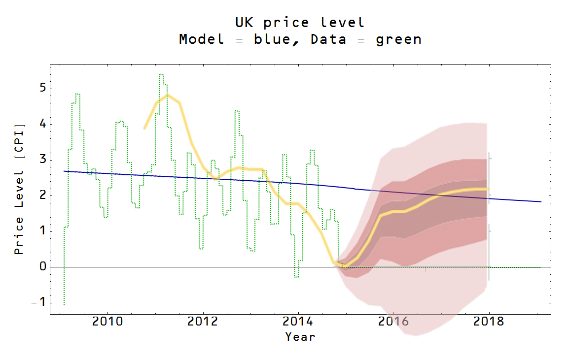
I was excited to see new forecasting from the new Bank of England blog (H/T to Simon Wren-Lewis), but unfortunately (for me) the result is completely consistent with the information equilibrium model. Since they agree and future data will not help decide between them, I thought it wasn't worth the effort of digitizing the graph and combining the data properly. Therefore I did a cheesy graphical plot overlaid on the results from here:

I used the second scenario where ELB was set at 0.5%, but it largely doesn't matter which one is used.