The baby-sitting co-op as an information transfer model

Paul Krugman has called the baby-sitting coop -- see here for original paper [pdf] -- his "favorite economic parable". It explains how recessions can be the result of poor monetary policy, that a lack of money (or in this case, baby-sitting scrip or coupons) can lead to lower output (fewer baby-sitting jobs). I've talked about it briefly before here. Let's put this parable into a formal information transfer model. Start with information equilibrium between the scrip (S), each coupon good for 30 minutes of babysitting, and the babysitting jobs (B).

P : B ⇄ S

Note that a babysitting job can potentially cost several coupons. That is our shorthand for a differential equation (see the paper) that has the solution (in general equilibrium):

B/B₀ = (S/S₀)ᵏ

The 'price level' is:

P = k (B₀/S₀) (S/S₀)ᵏ⁻¹

With this model, we have supply and demand curves in partial equilibrium where X stays near X* on the time scale that Y (the other process variable) changes (see the paper, with ΔX ≡ X - X₀):

Already we have some basic mechanics described in the paper and by Krugman:

• Depending on the value of k, the price level could be stable (k = 1), rise (k > 1, inflationary pressure) or fall (k < 1,  deflation)
• If scrip S falls, then babysitting B will fall in general equilibrium. Printing more scrip will allow babysitting to rise.

However, there is another bit of dynamics not captured in the mainstream economic model version that is present in the information transfer framework. It's called non-ideal information transfer. In general, the information in the spatial and temporal distribution of babysitting jobs is greater than the information in the spatial-temporal distribution of scrip (not everyone who wants to babysit can babysit) so:

I(B) ≥ I(S)

When these are not equal, I write this as an information transfer (not information equilibrium) relationship:

P : B → S

And the best we can do is put a bound on the non-ideal price level P*:

P* ≤ k (B₀/S₀) (S/S₀)ᵏ⁻¹

And if B* is the non-ideal level of output and P is the ideal price level, then

P* S/k = B* ≤ B = P S/k

Which means you can have a recession without it being caused by a lack of scrip. And this should actually happen sometimes. If you say there are a lot of time periods (say weeks) and a lot of people in the babysitting coop, even random behavior will tend to saturate this bound. But occasionally, it will be less even if there is sufficient scrip. It could look something like this:

The line at 100 represents information equilibrium level of output B. At time t = 150, we have B* ≤ B (a recession) due to non-ideal information transfer. Now it doesn't have to be random behavior causing it (it still could be) -- it could be a broken market or some complex behavior such as a subset of the coop deciding to go out all at the same time. Or everyone works for the government and there's a shutdown (the coop story was originally in Washington DC).

Also, even the non-ideal information transfer could be alleviated by a temporary increase in the level of scrip (which moves the information equilibrium bound up):

The babysitting coop is traditionally used as an example of how nominal shocks (to the quantity of money) can have real effects on output, and how monetary policy can be useful in setting things right. The information equilibrium picture reproduces this basic picture. However it adds that recessions may also be caused by other factors (financial panics, wars, market failure, human behavior) that have nothing to do with monetary policy. Instead of the financial crisis being caused by tight money in 2008, it might not have been the Fed's fault at all.

Basically, the information transfer framework says that things like recessions may not arise out of the behavior of rational agents (which tend to produce information equilibrium results).

The impotence of great men

This just seemed kind of odd to me:

This is my personal favorite from the Fed's long history of caving to political pressure. https://t.co/d6fBI4jvax pic.twitter.com/Xbmg1Nxqtw

— Binyamin Appelbaum (@BCAppelbaum) November 12, 2015

That must have been some shove for it to have had an effect for the next 15 years, 10 of which Martin wasn't even in office. So interest rates after 1965 should have been low, right? Actually, they went up (see the paper for the IT model; this form uses the same parameters for short and long term rates):

Overall, rates for the next few years were basically where the IT model said they should be. In fact, they were where they would have been predicted to be by the IT model from data up to 1963 extrapolated out all the way until the late 1970s (the oil shocks weren't predicted by the IT model). So neither Johnson nor Martin really did anything.

The 60s and 70s was a time when 'loose money' tended to send interest rates higher (due to the income inflation effect, as described by Milton Friedman), not lower. This is the general monetarist view that the IT model agrees with (at least until the 1980s). The impact of monetary expansion is positive in the 60s and 70s:

The IS curve had yet to become downward sloping (see here for a neat picture).

So in a sense, Martin and Johnson had no idea what they were doing. And we should be glad they didn't! They could have tried to keep interest rates low by stifling the growth prospects of the US -- reducing the money supply or not expanding as fast. They could have targeted 2% inflation like a laser. The required counterfactuals are draconian. We would have had the GDP per capita of Jordan today.

PS Here's the full interest rate graph (dashed box is shown above):

Is micro stickiness enough?

Many people look at this diagram from the SF Fed (see the discussion here) and see evidence of sticky wages at the micro level:

That spike at zero wage change changes from 12% to 16% and the result is 10% unemployment and a recession. Or so says Scott Sumner today, Paul Krugman in 2012, and commenter Bill here.

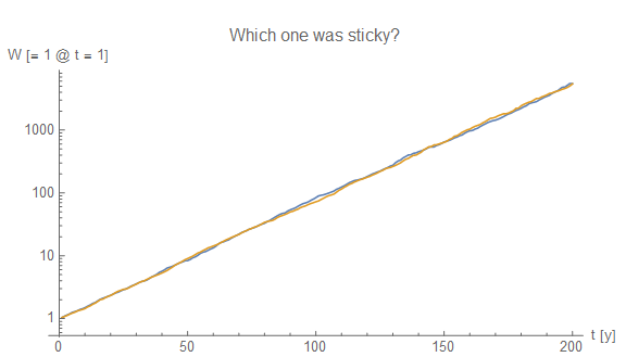
The question is -- can you tell the difference between the path of aggregate wages using those two empirical distributions to generate wage changes for the population? Not really. Here is the empirical distribution:

And here are several aggregate paths generated from that distribution:

Hard to tell, right? The blue line is the sticky one. And that's after 200 years of one being in a recession and one not! (The distribution from the SF Fed used annual changes, so each time step is a year.) It's only a few hundred people, not the millions in the labor force. So what would we expect if we did look at millions of agents? Here are the empirical distributions generated from more points:

The difference in the average of these two distributions is about 0.1 to 0.2 percentage points, so the difference in total aggregate wage change between populations with these two distributions is about 15 billion dollars = (0.2% x 7 trillion dollars). The US economy suffers a recession -- losing a several percent of GDP -- because the market cannot unstick 15 billion dollars?

That's why I think it's not the micro-stickiness of the zero bin, but rather the macro stickiness of being unable to coordinate a change in the whole distribution. The zero bin does contribute! In the previous link, it seems the observed 4% change in the zero bin would account for about 2% of the 8% NGDP loss (but from the entropy mechanism -- not lack of adjustment, they could all jump in the 1% growth bin or 5% growth bin and get the exact same effect on economic entropy that I wrote about again today). So the total effect looks like it's a bit of micro stickiness (but not for traditional economic reasons), but mostly macro stickiness.

Internal devaluation and the fluctuation theorem

File under speculative theory

Cullen Roche mentioned Greece today and that inspired me to take on internal devaluation:

... Greece ... exists in a single currency system with no floating exchange rate.  Greece is experiencing the equivalent of a gold standard style “internal rebalancing” where they suffer through a long sustained deflation that makes their economy more competitive.

For the standard economic narrative on this subject, here's Paul Krugman.

And here's why I think it might be such a difficult grinding process in terms of the information transfer model. In the paper I discuss how changes in nominal output (ΔN) are like the second law of thermodynamics for economics. In an ideal world where humans didn't act in concert (i.e. panic after a major stock market crash), we would have (on average, with a large economy):

ΔN ≥ 0

Atoms in an ideal gas don't suddenly decide to go to one side of the container (reducing entropy ΔS < 0), but humans can and will decide they want to get out of the stock market all at the same time. That allows ΔN < 0.

However even in thermodynamics you can have ΔS < 0, but only on a small scale. For microscopic engines, you can get the equivalent of an engine running backwards, sucking in exhaust and producing fuel (and it is relevant for biological machines like a ribosome or a flagellum). It's called the fluctuation theorem. You derive it by looking at the evolution of phase space going forward and backward in time, and the picture you should have in your head is something like this from Sevick et al:

The fluctuation theorem predicts a specific form of this violation of the second law of thermodynamics -- essentially an exponentially decaying function (which is actually observed, see e.g. here). Now I haven't formally proved that this carries over into economics, but if ΔN is analogous to entropy then the picture we have is like Figure 20 from the paper:

The green highlighted region indicates the strong violation of the 'second law' where ΔN < 0 due to panics and 'herd behavior', but some quarterly falls in NGDP would be consistent with a 'economic fluctuation theorem' (red highlighted region). In this picture, it is this piece of the distribution that would be analogous to the process 'internal devaluation'.

Does this offer any additional insight into macroeconomics?

Well, for one thing, it means that internal devaluation is easier for a smaller economy than a larger one. It is easier for a ribosome to operate backwards (thermodynamically) than a car engine.

In general, it should be a slow process since that region is exponentially small compared to the full distribution.

Additionally, for a small economy generally with an IT index k > 1, internal devaluation should also result in more deflation than for a larger economy with an IT index k ~ 1. Note that Paul Krugman has indicated that the lack of deflation was a puzzle (although Japan did experience deflation, so this isn't cut-and-dried).

Checking it twice (GDP and GDI)

Jérémie Cohen-Setton links to a new Fed report [pdf] about how some published results change if you use NGDI instead of NGDP; they find:

Estimating models using GDI, both with the GDI data originally available to the authors and with revised GDI, instead of GDP generates larger differences in results than those obtained with revised GDP. For 3 of 23 papers (13%), the results we obtain with GDI are qualitatively different than the original published results.

So I thought it would be good to check some IT model results using this method. I checked this post, and I basically get the same result:

And I checked this post:

It checks out so far. I'll continue to check these two independent measures of nominal output in the future.

Scooping the Financial Times

Martin Sandbu this last week in the Financial Times (H/T Jérémie Cohen-Setton here):

There is a simple idea that frames some of the biggest economic questions of our time and helps to clarify the positions and the stakes in the deepest disagreements over policy. It is that the “[Wicksellian] natural rate of interest” has fallen sharply; what you believe about why this may be determines much of what you believe is the appropriate policy response.

I wrote this two months ago:

The macroeconomic theory everyone seems to be working with (still) is the Wicksellian natural rate of interest. Paul Krugman mentioned it today. It really does create a unifying picture the various views of quantitative easing. Imagine it as the last common ancestor of Austrian, Keynesian and monetarist theories of economics.

Get yer hot takes at Information Transfer Economics first! Without the pink background ...

Temporal shapes of discount factors and utility functions

Update: Better title: "Angels dancing at the end of time"

In John Cochrane's paper [pdf] on neo-Fisherism, he posits that the representative household maximizes:

$$
E \left[ \sum_{t = 0}^{t = \infty} \beta^{t} u(c_{t}) \right]
$$

This is not an unusual equation and I'm not singling Cochrane out. It just happened to be the first place I saw this after writing this post. However, this is an interesting mathematical object. The only thing that makes the limit $t = \infty$ make sense is that there is an implicit time scale (call it $t_{\beta}$) over which the discount factor $\beta$ falls to zero. And $\beta$ exists in order to make the infinite sum convergent. There is also economic growth, so there is another timescale $t_{c}$ introduced through the consumption $c_{t}$. Let's pass through to continuous time and explicitly show our scales:

$$
E \left[ \int_{0}^{\infty} dt \; \beta(t/t_{\beta}) \; u(c(t/t_{c})) \right]
$$

This has units of time, grows when $t_{\beta}$ grows (less discounting of the future) and gets smaller when $t_{c}$ grows (the economy is slower growing because the growth rate $g \sim 1/t_{c}$), so it must be [2]:

$$
E \left[ \int_{0}^{\infty} dt \; \beta(t/t_{\beta}) \; u(c(t/t_{c})) \right]= \alpha \frac{t_{\beta}^{2}}{t_{c}}
$$

where $\alpha$ is some $o(1)$ constant dependent on the specific temporal shapes of the utility function and the discount factor [1].

The discount rate $1/t_{\beta}$ should be a deep parameter in the Lucas sense (based on how human behavior discounts the future) and the growth rate scale should be a deep parameter of the economy. So we should find the expected value at the top of this post depends primarily on the temporal shape of expectations (i.e. changes in $\alpha$).

It should therefore primarily depend on the temporal shape of expectations and discounting when exposed to shocks, since temporary shocks shouldn't change deep parameters (this is not a necessary restriction as we'll see below).

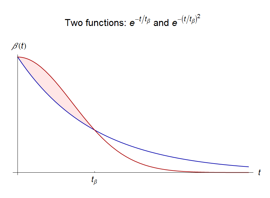
For example, I can cause the representative household's expected utility of consumption to fall in half by switching from $\beta \sim \exp -t/t_{\beta}$ [1] to $\beta \sim \exp -(t/t_{\beta})^{2}$. The difference comes from times $t > t_{\beta}$ -- far out in the tail of the distribution -- because for $t < t_{\beta}$ the second function actually has less discounting (the red curve is above the blue curve for small $t$, shaded region):

So you can see how expectations and discounting at 'infinity' can create results like Cochrane's and Woodford's.

In general, however, Cochrane's objective function maximized by the representative household (at the top of this post) gives us a really great way to organize several different takes on our current macro situation in the US:

• The neo-Fisherite view seems to be mostly about $\alpha$. I may be wrong about this, but that is what I am seeing.
• Both Paul Krugman's liquidity trap and Scott Sumner's NGDP are about changing the scale $t_{c}$ (Krugman says changing expected $t_{c}$ is hard without fiscal stimulus, Sumner says the central bank can set whatever expected $t_{c}$ it wants). Low interest rates are due to not just low growth in the short run (a change in $\alpha$), but low expected $t_{c}$.
• There don't appear to be any takes that directly modify the discounting scale $t_{\beta}$. However, since there are only two scales, it really only makes sense to talk about one relative to the other (i.e. $t_{c} > t_{\beta}$ or $t_{c} < t_{\beta}$). Therefore a change in $t_{\beta}$ could just be re-interpreted as a change in $t_{c}$.

Footnotes:

[1] Note that $\alpha = 1$ when $u(c) = \log(c)$, $c \sim \exp t/t_{c}$ and $\beta \sim \exp -t/t_{\beta}$.

[2] This is a fun trick we learn in physics called the "what else could it be?" argument (it's basically dimensional analysis). For example, the energy of an bound state of the Hydrogen atom, if $m_{p} \gg m_{e}$ kind of has to be

$$
E \sim - k \alpha^{2} m_{e} + o(m_{e}/m_{p})
$$

where $k$ is some constant (turns out it's $k = 1/2$). The only energy scale is the mass of the electron (times $c^{2}$ but we're using 'natural' $\hbar = c = 1$ units, so mass is energy) and it's an (observable, not just an amplitude) electromagnetic interaction so you need two factors of $\alpha$ (coupling the electron to a photon and the photon to the proton). There is no other sensible combination that can come together to create something with the units of energy to be an energy eigenvalue. [$\alpha = e^{2}/4 \pi$ is the fine-structure constant -- there is a factor of $e$ (electric charge) coupling for the electron to the photon and the photon to the proton, and this is squared to get an observable, not an amplitude, proportional to $\alpha^{2}$]

On limits

One thing to keep in mind when using mathematics to describe physical reality is that you have to be very careful about taking limits. In pure mathematics it's generally acceptable to send a variable off to infinity, m → ∞. If you are using mathematics to describe physical reality, then m might just have 'dimensions' (aka 'units') so sending a dimensionful number off to dimensionless infinity (or zero) can give you weird results.

Generally, if, say, m is a mass (with units of kilograms) the only way you can send it off to infinity or zero is to have another scale (say, another mass M with units of kilograms) to compare it to. You can send m/M → ∞ or m/M → 0 ... or better yet, as physicists tend to put it: m/M >> 1 or m/M << 1 (i.e. m >> M or m << M).

I do my best to be very careful about this (I probably have made some mistakes). However, I don't think economists care about this at all. For example, Paul Romer and Robert Lucas both take limits where time T and a time scale (1/β, where β is a rate) go off to infinity simultaneously. In pure math, this produces an issue of almost uniform convergence; however, if you're using math to describe physical reality then it is nonsense to send these two dimensionful scales off to dimensionless infinity simultaneously. A (possible, since it was EJR) econ student also had no idea about this, which makes me think this attitude is very widespread. The only sensible thing you can do is look at T β >> 1 or T β << 1. Other limits are nonsense.

Nick Rowe doesn't seem to have a problem with sending dimensionful numbers to dimensionless infinity either (which I wrote about yesterday), sending time steps dT to zero when he should really be looking at the relationship to the other physical scale in his theory -- the delay in the onset of the end of fiscal stimulus dt. This carelessness creates nonsense results.

Noah Smith, John Cochrane and Michael Woodford (see Noah for one-stop shopping, and see slide 30 of Woodford's presentation [pdf] [1]) all make this same error when talking about neo-Fisherism in terms of permanent rate pegs and expectations infinitely far in the future. And if Woodford is considered the Ed Witten of economics (per Noah in the link above), that doesn't bode well for any economist knowing about how to use math to describe reality. It also makes me think the whole neo-Fisherite view may just be an artefact of poor dimensional analysis (something that I will be looking into ... )

The problem is that economists don't see this as an issue. And they don't seem to take kindly to physicists trying to tell them what to do. When Chris House says "[Physicists'] mathematical abilities are actually not that much better than most economists (if they are better at all)" my spidey sense starts suggesting the reason is probably Dunning-Kruger [2]. The second paper on his list on his website ("Layoffs, Lemons and Temps") has a individual firms with "production function[s] with the usual properties" which in the footnote contains two nonsense limits where the number of workers n goes to zero and infinity ... treated as if it's an everyday assumption (even relegated to a footnote). They are in fact everyday assumptions in economics (called the Inada conditions)! The only sensible limits in that case would be (for instance) n/N >> 1 or n/N << 1 where N is the number of firms (in English, a few firms have a large number of workers versus many firms have a small number of workers). Another way would be to compare to the population size (does everyone work for a few companies, n/P ~ 1, or do very few people work for the same company, n/P << 1). I don't think this impacts the results of House's paper, but it is careless mathematics. At least the Inada conditions are described in terms of a pure mathematical function with dimensionless inputs.

Update 11/9/2015:

Even if the reason for finite number of belief updates in footnote [1] is that they cost some amount of money dm (or people are just n-smart), you still can't send dimensionful time T to dimensionless infinity when things happen in your model that take finite amount of time (or have some finite timescale such as the decaying functions on Woodford's slide 26). The version where revisions take a finite time dt is just one possible way to make the limit make sense -- not necessarily the only way. It's sort of like the example above with Chris House's paper where I used N and P. The issue is that there has to be some scale that the number of workers n is large compared to be it the number of firms or the total population, and there has to be some timescale that time T is long compared to.

Footnotes:

[1] Woodford takes two limits of n → ∞ and  T → ∞ where n is the number of 'belief revisions'; these revisions obviously take some finite time dt (or else you could do an infinite number of revisions instantaneously), so the only sensible (in the sense of using math to describe reality) limits are n dt/T >> 1 or n dt/T << 1. The first says that belief revisions take longer than the time horizon of the interest rate peg (interest rates stop being pegged before you fully revise your beliefs -- which doesn't seem like a very long peg); the second says you revise your beliefs to a high order before the interest rate peg ends (which actually makes more sense). The limits that Woodford takes (n dt → ∞ and T → ∞ simultaneously, in both orders) don't make any sense.

[2] I've sort of come through the rabbit hole on this one. In my first forays into econ, I basically thought economists were just fine with math. I tended to defend econ from usurping physicists (here and here). But these limit problems (in  a paper by preeminent economist Michael Woodford, no less) coupled with Paul Romer's diatribe against mathiness and Nick Rowe on the RCK model makes me think that maybe economists don't really know what they are talking about.

Expecting more precision than possible

Diane Coyle has taken her crusade against GDP (as a measure) to the NYTimes OpEd page. I don't have much issue with it in general, however she claims:

Growth forecasts for gross domestic product in the United States at the end of this year vary from about 1.75 percent to 3 percent — a good measure of the lack of consensus.

Does this reflect a lack of consensus? I did some simple linear extrapolations in the IT model and looked at the error in the estimate of 2015 Q4 RGDP (i.e. propagating error in the prediction of PCE inflation and NGDP to RGDP) to get a handle on how big a 125 basis point variation stacks up. Here are the extrapolations:

That's 1-σ (standard deviation), so we'd expect it to be outside that range more than 30% of the time. What we end up with is an estimate between 0.7% and 4.9% with roughly 70% confidence -- a 420 basis point error band.

Even casual observation of the raw data tells us the 125 basis point spread (black rectangle on the second plot) is remarkably tight. My 420 point band would be more indicative of a lack of consensus!

The truth is that precision to less than a percentage point may not even be possible. It seems Diane Coyle is setting up economic forecasts to fail.

If a model result is silly, question the scope before questioning the model

Awhile ago I wrote a bit about scope conditions (or rather the lack of them) in economics. Nick Rowe provides us with a good illustration of this problem with his post on the effects of a delay in ending fiscal policy in New Keynesian models. After reading his post, I commented:

So wait: expectations of a delay in returning taxes to normal produce a change in expectations from an expected temporary change in tax rates to an expected permanent change in tax rates? 

Can we add in rational expectations of an expected delay (obviously the government doesn't stop on a dime), so that people don't revise their expectations of a permanent/temporary tax change based on a delay in returning taxes to normal?

I was being a bit tongue in cheek; the result that an infinitesimal delay in the end of fiscal stimulus changing people's expectations of fiscal policy from temporary to permanent (and thus changing the sign and magnitude of the multiplier) is, in a word, silly. It's a bit like a child thinking that because class didn't let out at exactly 3pm, class will instead last (literally) forever.

You could cure this by saying that the theory is valid for government delays dt << 1 so that t + 1 ≈ t +dt  + 1. But then, that's the kind of thing that should have been a scope condition in the theory in the first place.

Nick says:

How long is "one period"? It's as short as you want it to be.

No; that is false. For one thing it can't be shorter than the Planck time. In general, it can't be shorter than the time it takes for light to traverse the entire country in question and return to that point (about 20 milliseconds for the US). It takes a few milliseconds for sensory input to register in our brains.

Less sarcastically, there is a definite period of time over which rational expectations can reasonably take hold. Quarterly NGDP data from the BEA isn't released until a month after the quarter ends. Budgets generally have annual cycles. It takes months (weeks, on rare occasions) to get bills through the US congress. There obviously exist timescales over which macroeconomic and government processes happen.

The New Keynesian theory should have something to say about what "one period" means (it seems to be quarterly from various models I've seen). It should also have some kind of estimate about the relative size of the timescale of government actions (dt) and the reaction of the macroeconomy (dT). Is dt << dT? In that case Nick's analysis is silly, not the result. Nick implicitly assumes dt >> dT (the macroeconomy reacts faster than the government). Maybe that is true (data would help), but it is obviously not a region of validity of the New Keynesian model -- we know this because you get silly results like sudden shifts between fiscal policy being contractionary or expansionary based on a one month delay in changing marginal tax rates.

It's a bit like saying electrodynamics predicts atoms will radiate all their energy and collapse so atoms must not exist. But electrodynamics is not valid for cases where ћ ~ dx dp; you need quantum mechanics. That is to say you need to understand the scope conditions of your theory. If you've found a problem, the problem could well be that you've applied the theory incorrectly.

Funny enough, this is very similar to the mathiness issue between Paul Romer and Robert Lucas. The issue has the same form: Lucas's model is assumed to have infinite scope for its variables and Romer says Lucas's model has different limits if 1/β >> T and 1/β << T where 1/β is the timescale for innovation and T is the observation time of the economy. Those two limits have different model interpretations: innovation is slow (so it never happens) versus innovation is fast (so it has already happened). These are entirely different kinds of worlds.

But no one in economics seems to care about scope [1]. Nick Rowe is just fine with the idea that the New Keynesian model is valid for both extremely fast and extremely slow changes in government fiscal policy. He says the extremely slow version gives us silly results so we shouldn't trust the extremely fast version either. 

But you can't extrapolate from one limit to the other. The more logical conclusion is that the extremely slow version is out of scope of the theory.

Footnotes:

[1] Don't just take my word for it; Noah Smith says:

I have not seen economists spend much time thinking about domains of applicability (what physicists usually call "scope conditions"). But it's an important topic to think about.