Floating information sources, physical laws and volition

Peter Dorman brings up an interesting point:

... models of the macroeconomy incorporate monetary policy as just another component of “the economy”, along with the behavior of households and firms. [They] include the reaction functions of monetary authorities as determinate behavioral foundations of how the economy works; there is no corresponding behavioral rule on this fiscal side. 

Back in the days of IS-LM with a fixed money supply (fixed for some unmentioned reason by an almighty central bank), the model consisted of behavioral responses in the money and goods markets, leading to a predicted outcome, equilibrium levels of national income and interest rates. 

... you plugged in a policy choice and it told you how the economy was supposed to respond. 

Now it’s different, at least on the monetary side. In the new versions of IS-LM and AS-AD, as well as the more elaborate models in the professional literature, monetary policy is inside the model. The choices of central bankers are built in. You may have interest rate targeting, inflation targeting or some version of a Taylor Rule, but in all of them the monetary choices themselves are predetermined.

This is effectively the choice between a "floating" information destination and a "constant" information destination (in the market P:NGDP→MB) in the information transfer framework (see here or here). "Floating" means the Fed uses some target or rule, effectively looking to the market like any other business building widgets. "Constant" means it just builds its widgets at some fixed rate. In the former case, the Fed's behavior may be "constrained" (as Dorman says) but it's the kind of constraint that follows from there being lots of dollars (basically, the law of large numbers) and has little to do with volition on the part of the Fed. We don't say an ideal gas is "constrained" from doing what it wants by the ideal gas law. The physical system follows the ideal gas law. These Fed reaction functions are more like Maxwell distributions; Maxwell distributions don't constrain the movements of atoms (which can have any speed) -- they are the result of gazillions of atoms following the laws of physics. These Fed reaction functions don't constrain how the Fed increases the monetary base, they are the result of billions of dollars interacting with the market. The information transfer model with a floating information destination makes minimal assumptions about these functions and just assumes at a fundamental level information in is equal to the information out, or one level up, supply and demand is at work.

In the case of a constant information destination, where the Fed just sets an interest rate or targets a monetary aggregate, the aggregate demand (NDGP) is the only thing doing the reacting. This case generally leads to accelerating inflation.

Why isn't there a government reaction function (asks Dorman)? My best answer in this framework: Because the government (G) is only a piece of aggregate demand NGDP = C + I + G + (X-M). If G were a floating information source then it would just mix in with C, I, X and M as floating information sources leading to NGDP being a floating information source. If G were a constant information source (basically how it is treated), we'd still have C, I, X and M as floating sources that would still allow NGDP to adjust to the monetary base MB.

Supply side reforms didn't accomplish anything

How's that for a provocative title? Scott Sumner is back with his claim that supply side reforms helped keep the US and the UK growing faster than other countries in the 1980s. More precisely, he believes that while most large economies showed slower growth after the 1970s, the reduction was less in the US and UK because of Reagan/Thatcher supply side reforms such as tax cuts on income and capital gains and moves to control inflation.

I will argue that only the moves to control inflation are responsible (monetary policy) and the resulting relative growth rates were actually baked-in immediately after WWII.

First, let's look at the information transfer index for several countries:

As you can see the information transfer index (IT index) is lower for the US and UK relative to Japan and the EU which generally means that increases in the monetary base have more impact than for countries with higher IT index. A better way to look at it is in normalized space:

You can see the information trap criterion (∂P/∂MB = 0) line (black dotted curve). In general, low IT index and low normalized monetary base (see the link before this graph) mean you are farther from the information trap criterion and so monetary policy is more effective (increases in MB have a projection along the GDP direction, growing the economy).

What does this mean? It means that if these countries go to control inflation by reducing the growth of the money supply and other monetarist reforms, the resulting GDP growth is going to be higher in countries with low IT indices and monetary bases and lower in countries with high IT indices and monetary bases for similar levels of inflation.

I will demonstrate this with US data. I first extracted the non-monetary component of GDP (aka "shocks") growth like I did here. I then "grew" the economy from 1960 by inflating according to the growth in the monetary base and adding the shocks over tiny steps. With this procedure, you basically recover the path of NGDP from the start point in 1960. I show this in the following graph (solid line) along with two economies I "grew" with the same economic histories but a smaller IT index as well as a larger one (the higher and lower dashed curves, respectively):

The first thing that is apparent is that the lower IT index has higher growth and vice versa given the same economic histories. A second interesting observation is that the quantitative easing undertaken in 2009-2011 and beyond would have actually boosted the economy if our IT index had been lower and the recession would have been worse if the IT index was higher.

It is likely the difference in growth rates among countries after the supply side reforms of the 1980s was entirely monetary. The tax cuts likely did very little. And why was the US IT index and base so low in the first place? GDP growth during WWII.

For completeness, here are the curves in normalized space and the analogous graph of the IT index shown at the top of this post:

Economy in the U.K.

I know what I want and
I know how to get it

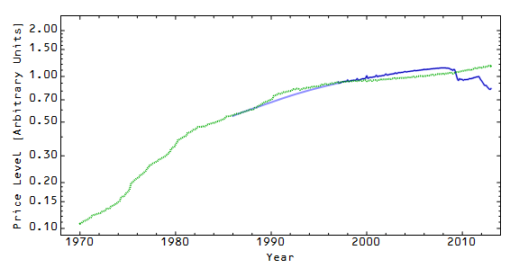
Although I tried it already, I thought I'd do this for the UK. I re-used some the data I used in this attempt, however the problem with that was that there was insufficient data from the period before the recent crisis so the fit over-weighted it. The reserves component of the base only goes back to 2006, and the currency component only goes back to 1996, so in reality I was only working with data from 2006-2013.

Therefore I decided to use some extrapolation (linear extrapolation in log space) as well as (for the first time) actually trusting my interest rate model in order to determine the monetary base further back. It worked when I used a fit to US interest rates from 1960-2013 on data from 1930-1960, so I figured I could extrapolate the monetary base data back to 1986 through the interest rate data from FRED.

I did it in two stages. First, I did a linear extrapolation (in log space) of the reserve balances data before 2008 back to the beginning of the currency data (1996). This formed the basis for a fit to the interest rate:

The dashed blue curve represents using the interest rate model to extrapolate the 1996-extrapolated data (solid blue curve) to 1986. The 3-month LIBOR data is green. The resulting monetary base is shown here:

Green is actual reserve balance data, red is actual currency data, dark blue is the 1996-extrapolated data (the sum of the currency and extrapolated reserves) and light blue is the interest rate 1986-extrapolated data. Using this monetary base, we can now show the model (blue) of the price level (CPI data less food and energy, green):

This is an improvement over the original result, but still shows a deviation for the current crisis that is not as apparent in the US model. We'll see how this progresses over time. Maybe this is real and deflation will set in in the UK. Inflation is in fact falling. However this more likely represents residual model error.

What is interesting is that if we plot the path in NGDP-MB space, the information trap rate in the UK seems to be about 3% (it is 2% in the EU, 1% in Japan and 0.1% in the US):

The red lines represent constant interest rates, the dashed black line is the information trap criterion (∂P/∂MB = 0) and the actual path (well, extrapolated path) is shown in blue.

Update 21 January 2017

Another more recent post with a better model is here.

Apparently monetary offset only offsets things you don't like

For a rather humorous exercise in data analysis leading to confirmation bias you should check out the linked article presented in Scott Sumner's post from the other day.  Kevin Erdmann makes the rather paradoxical assumption that the integral of a distribution over one domain can be considered to be predictably proportional to an integral over a different domain when the distribution itself is changing (a fact of which he is totally aware and is trying to study). I'd like to talk instead about Sumner's response in which he says that unemployment is "over-determined" in the sense that if you tried to tease out the different factors leading to unemployment you could find ... well, let's just quote Sumner ... "multiple factors are each powerful enough to explain most unemployment".

That is excellent news. Everyone's model is cool!

Of course, Sumner has to simultaneously believe that the level of aggregate demand is set by the central bank and that unemployment insurance causes some extra unemployment, therefore unemployment must be overdetermined: UI can cause more unemployment than there would be otherwise but take it away and the overall level of employment, which is set by the central bank, would still be the same. Another way to put this is that somehow UI causes extra unemployment but the getting rid of UI is fiscal policy subject to monetary offset. Or yet another way, UI is magic.

Since apparently no one knows how to logically approach a problem anymore, I will demonstrate. Now you might not believe the underlying model I'm using, but at least this approach is coherent.

How does Extended UI affect the unemployment rate in the Labor Supply market?

I put together a model of the labor market in my effort to construct Scott Sumner's model. The basic premise is that the price level detects signals from the aggregate demand to the labor supply. Now these signals include individual decisions to sit around on the dole, leave the labor market, get a part time job, retire and every other possible reason someone would or wouldn't be considered a member of PAYEMS. This model does a good job of describing the price level:

It does an even better job (at least for economics) with Okun's law (see the model link for the derivation):

So if I was to ask the question: Does EUI increase the unemployment rate? My first task would be to address whether the current unemployment rate was consistent with Okun's law. Here are the data points and the model curve:

And here are the residuals and a 2-sigma error bar:

If we look at the residuals as a time series we can see that there is nothing special about this recession: 

EUI started in 2008. There is always a deviation from Okun's law at the start of a recession (there is a statistically significant layoff over-reaction to the actual drop in RGDP) but the subsequent labor supply growth rates are exactly what we expected with no change to the relationship over the entire period from 1960 to today when EUI was not in effect. If we had seen a deviation then there might be a case to be made but this 1% order effect is deep in the noise.

PS My favorite rationale for why people are unemployed:

Because--more young adults are becoming unemployed on account of they can't find work! Basically, the problem is this: if you haven't got a job, then you outta work! And that means only one thing-- unemployment!

Top ten successes of the information transfer model

(1) Explaining supply and demand: If you set up a description of an information transfer process moving information through a channel from a source to a destination and make some identifications (the demand as the information source, the supply as the information destination and the price as a detector of a signal sent from the demand to the supply), you basically get out fundamental economic supply and demand logic including supply and demand diagrams (another way to visualize diagrams is here). I've used the notation Price:Demand→Supply to describe these models of a market.

(2) Modeling the price level: This is basically done with a quantity theory of money, using the information transfer framework with a market P:NGDP→MB (the price level detects signals from the aggregate demand or NGDP to the monetary base). The major results for the US are here. The fit to RGDP growth is rather remarkable. I also fit the data for the entire period from 1929 to 2013 using three monetary policy regimes with great success (market-based systems before and after WWII, with a pegged interest rate model in between). More on monetary regimes is here including a theorem that increasing the monetary base will eventually lead to an information trap (basically a liquidity trap). One of the key pieces of the model that allows such success in fitting the data is the way the behavior of money as a unit of account is incorporated in the model via a varying information transfer index. In a sense, the monetary base is the number base you count the GDP in much like binary is the number base you count data in, but in the latter case the base is fixed at two. It also works for the EU and Japan.

(3) Modeling interest rates: The best result was the same fit the data from 1960-2013 also fit 1929-2013. Overall, the simple model (derived from the IS-LM model) does a good job of describing the US, Japan and the EU.

(4) Modeling Japan's lost decade: Japan's sluggish economy and immunity to inflation is a major problem in economics. The information transfer model describes the price level and interest rates and the major conclusion is that Japan is in an information trap, a condition where monetary policy has little influence on the price level.

(5) Deriving the quantity theory of money (and explaining deviations): The basic equation in the information transfer model for the market P:NGDP→MB looks like the equation of exchange. You can also derive the major result of the quantity theory from the model (specifically that for high inflation, the rate of monetary base growth equals the rate of inflation or r = i). But it is even better than that. The information transfer model explains the deviations at low inflation from the basic r = i picture.

(6) Deriving the IS-LM model: The supply and demand framework allows a straightforward derivation of the curves in an IS-LM diagram.

(7) Okun's law: A relatively straightforward application of the model building capability of the information transfer model allows us to build a market P:NGDP→LS (price level detecting a signal from the aggregate demand to the labor supply) that recovers Okun's law.

(8) Walras' law: This follows from the supply and demand model via some algebra.

(9) Explaining how the EU can be in a liquidity trap but not at the zero lower bound: Keynes' original work allowed a liquidity trap to occur at any interest rate. Later economists argued that it could only occur at zero interest rates (as they can't be lowered). Now Paul Krugman argues that the EU is in a liquidity trap even though EU rates are not actually zero (as Scott Sumner points out); Krugman's explanation is that they are close enough. The information transfer model shows that the liquidity trap rate is actually a function of GDP and the monetary base. For example, it is about 2% for the EU, 1% for Japan and 0.1% for the US.

(10) Explaining the history of economic thought in the US since the early 1900s: Since the path of GDP and the monetary base give us interest rates and the price level since the early 1900s, we can use the fact that the model appears to be a quantity theory of money and an IS-LM model at different times to understand the currents in the history of economic theory. In particular, we expect to get quantity theories before the depression (check) displaced by interest rate and liquidity trap theories in the 1930s (check), a resurgence of quantity theories in the 1960s-70s (check) and a return to interest rate and liquidity trap theories today (check).

Ch-ch-ch-changes.

I was re-reading this post (and the one Noah Smith links to in it) about what we mean by economic cycles, (or even how to extract the effects of policy changes; this seems like a bad way to do it) and thought I should update my take on it.

The procedure I came up (for what is essentially a quantity theory of money) is to extrapolate where the economy would be if the monetary base increased from time T1 to time T2 (which generally increases the price level) but GDP remained the same when adjusted for inflation. Call this point GDP0(T2). I then looked at the remainder when I took the difference GDP(T2) - GDP0(T2). Basically this is the distance the actual GDP is from the GDP you expected to arrive at given monetary policy. Graphically, the process is described here where I referred to that remainder as a "nominal shock". Here is a graph based on NGDP data (dark blue is a LOESS smoothing and red indicates recessions):

I also went back to this fit to all the data since 1929 (using GNP instead of GDP) and extracted these nominal shocks (the colors correspond to the different monetary policy regimes described in the link):

Six points

Borrowing a theme from my other blog Spittle-Flecked Ire (which I've been ignoring), I'd like to say these statements:

1. David Beckworth looks [at] a bunch of natural experiments on the efficacy of monetary policy at the zero bound ... [1] 
2. These three quasi-natural experiments indicate that there is much monetary policy can do at the ZLB. [2]

are based on exactly six data points across three countries. That is neither "a bunch" nor do they "indicate" anything. Here are the two data points for Japan:

It seems like confirmation bias. I still say RGDP growth will continue its post-2000 average for Japan,  its post-2009 average for the US, and its post-2009 average for the EU. These predictions are based on hundreds of data points (in fact, all available data).

For completeness, here are the four other points:

Analyzing the EU with the information transfer model

Today I analyzed the EU with the information transfer model and produced the analogous graphs from this post (the price level), this post (interest rates) and this post (interest rates, the liquidity trap and the information trap). The monetary base data came from here and the GDP, GDP deflator and interest rate data came from FRED. Altogether the story is similar to the US and Japan. The EU is in an information/liquidity trap. The interesting result is that this tests the hypothesis that the zero lower bound is not a necessary requirement to be in the trap. Scott Sumner frequently points out that the ECB is not at the zero lower bound (rates are at ~1%) as an argument against Paul Krugman and the liquidity trap. However, this analysis shows that the "liquidity trap" interest rate is almost 2% in the EU (in Japan it is 1% and in the US it is 0.1%).

First I will start with the price level fit (model in blue, GDP deflator data in green):

For reference, here is the information transfer index (quite high since the Euro's inception):

For fun, here is the 3D price level surface (again, model in blue, deflator data in green):

Now we come to the interest rate models. I used the discount rate, which roughly tracks the 3-month rate. There are probably some issues -- the ECB (and markets) seem to treat Greek debt differently than German debt so there is no overall "EU" rate -- but the fit does a decent job anyway (discount rate in green, model calculation in blue):

The money-graph behind the bold claim at the top of this post is last. The constant interest rate contours in (MB, GDP) space are shown as red lines, the information/liquidity trap criterion is shown as a black line and the path followed by the empirical data is shown in blue. The key takeaway is that the "liquidity trap" rate (given by the location of the black line given the current level of GDP) is almost 2%:

Addendum

I'd like to point out that the first graph is a non-trivial result; the Euro monetary base does not have a immediately obvious relationship with the price level:

Exit through the hyperinflation

Update 5/14/2015 

I updated the graphs at this link. It doesn't change any of the conclusions, so I'll leave this post unchanged.

In the last post I mentioned that I would look at accelerating inflation as a potential way to exit from a liquidity/information trap. First let me start with interest rates. The information framework describes the effective fed funds rate very well from the 1960s onward. In order to look at even earlier times, I looked at the 3-month interest rate instead (which is approximately equal to the Fed funds rate, and is shown in green) and added a few points I managed to get from a Fed paper on the Depression for the years 1929-1931 (green dots). Even without re-fitting the data to the entire 1929-2013 period (fit only to 1960-2013), I got a remarkable fit:

The model result is shown in blue. There is no "information trap" in the interest rate market model r:NGDP→MB, (NGDP standing in for aggregate demand, and MB being the monetary base) just a zero lower bound problem (they can be related in the sense that they happen at the same time).  Therefore the same parameters can be used for interest rates across the phase transition between the Depression and Post-WWII periods. However, if we look at the interest rate data we see the first sign of how a central bank can exit a liquidity/information trap and usher in that phase transition. In the highlighted region in the graph (World War II and afterwards), you can see the Fed pegged interest rates. That is key to leaving a path given by a market-based monetary policy and induces hyperinflation (or just accelerating inflation). In the information transfer framework, that is incorporated going from a floating, market-adjusting information source i.e. aggregate demand and destination i.e. money supply to a floating, market-adjusting information source and a constant, market-ignoring information destination.

This all means we need to use different models to form the complete story. We have P:NGDP→MB with market MB before WWII, statist MB during WWII and a return to market MB after WWII. In the graph below, I fit the models to the data before (red) and after (blue) WWII (from this post). The new result is adding the piece in the middle using the accelerating inflation model (purple):

This is a much better description than the original phase transition model. Since the 3D price level diagram includes what are basically three distinct models, they don't represent a single surface. I've shown them as patches in this figure (with the empirical data shown as a blue line):

One additional interesting result is that it is possible this non-market/statist/constant information destination (money supply/central bank) continued until the 1980s, at least in terms of the price level. One thing to recall is that the Federal Reserve Act was amended in the 1970s to include inflation as part of a dual mandate. With that legislation the market P:NGDP→MB goes from having a non-market information destination to a market destination. Why do I include this possibility? Well, the accelerating inflation model works well all the way up to the 1970s if you let it:

Although in that case the fit no longer works during WWII.

What does this exit via accelerating inflation picture mean for the US today? Well, it appears as though the Fed could peg interest rates a given time period (say, 10 years), markets be damned, and we would leave the liquidity/information trap. This rate doesn't even have to be zero as far as the model goes -- it could be 3%. That would be illegal (because of the dual mandate) so Congress would likely have to amend the Federal Reserve Act. This is politically impossible right now, so we're probably doomed to a Japan-like lost decade or two.

Interest rates and monetary policy or: Never reason from a price change

Scott Sumner has a great post up today. Great, in the sense that he lays out with some clarity how he sees interest rates (I will call these rules S1 - S4):

1. Moves toward easier money usually lower short term rates. The effect on long term rates is unpredictable.
2. Moves toward tighter money usually raise short term rates. The effect on long term rates is unpredictable.
3. Extremely easy money policies (hyperinflation) almost always raise interest rates.
4. Vice versa. [Which I have taken to mean "Extremely tight money policies (disinflation) almost always lower interest rates".]

But his immediate reaction (as well as Yglesias's) to the immediate reaction to the Fed's guidance that it won't start "tapering" violated his maxim to never reason from a price change.

So what does the information transfer model say about monetary policy and interest rates? I will make a list like Sumner did, but the interesting piece comes in when you recognize that markets don't know about the information transfer model. Hence the market reaction to easier money is always lower rates, but the long run depends on whether you are in a high information transfer (IT) index regime or not:

1. If the IT index is high, increases in the monetary base lowers interest rates (increasing MB causes NGDP to stay the same or drop slightly, decreasing NGDP/MB ~ r). Markets will also shift to lower rates as MB is increasing (perception of easier money).
2. If the IT index is high, decreases in the monetary base raises interest rates (decreasing MB causes NGDP to stay the same or increase slightly, increasing NGDP/MB ~ r). Markets will also shift to higher rates as MB is decreasing (perception of tighter money).
3. If the IT index is low, increases in the monetary base will raise interest rates (increasing MB causes NGDP to increase more, increasing  NGDP/MB ~ r). Markets will initially shift to lower rates as MB is increasing (perception of easier money) but the equilibrium will drift to higher rates over the long run.
4. If the IT index is low, decreases in the monetary base will lower interest rates (decreasing MB causes NGDP to drop, decreasing NGDP/MB ~ r). Markets will initially shift to higher rates as MB is decreasing (perception of tighter money) but the equilibrium will drift to lower rates over the long run.

High and low IT index is dependent on how close the economy is to the information trap criterion, and some of the reasoning can be understood from these two posts. I will call these rules I1 - I4. Let's review Sumner's rules in the light of the information rules:

1. Moves toward easier money usually lower short term rates. The effect on long term rates is unpredictable. This is because this case includes both I1 and I3. Markets like what they think is easier money, but the long run depends on whether the information transfer index is high or low. 
2. Moves toward tighter money usually raise short term rates. The effect on long term rates is unpredictable. This is because this case includes both I2 and I4. Markets don't like what they think is tighter money, but the long run depends on whether the information transfer index is high or low.
3. Extremely easy money policies (hyperinflation) almost always raise interest rates. This is rule I3. Sumner is basically recalling the 1970s here when the information transfer index was low. However this does not apply during the 1930s or since 2008. Sumner rationalizes this by saying money during the 1930s and 2010s is tight (see next rule) despite the massive increases in the monetary base (the increase is expected to vanish ... eventually).
4. Extremely tight money policies (disinflation) almost always lower interest rates. This is rule I4. Sumner believes this is the situation in the 1930s, the 1980s and now (his views are consistent with the information transfer model if the IT index is always low). Rule I4 only applies if the IT index is low, which works in the 1980s, but is incorrect in the 1930s and since 2008 since the IT index is high. We do not have "tight" money that is leading to low interest rates, we are in a liquidity trap which happens at low interest rates and monetary policy is ineffective: money is neither tight nor loose.

Another way to see this is by eras:

• The 1930s: Sumner says S4 explains. I say I1 explains. (We disagree on whether the Fed could intervene.)
• The 1970s: Sumner says S3 explains. I say I3 explains. (We agree inflation was a monetary phenomenon.)
• The 1980s: Sumner says S4 explains. I say I4 explains. (We agree that monetary policy brought inflation under control.)
• The 2010s: Sumner says S4 explains. I say I1 explains. (We disagree.)

I think this is also a good place to place to compare and contrast the information transfer model with two other views of our current situation:

Scott Sumner believes the current situation is like the US in the 1930s and Japan. Money is tight and the Fed could create expectations that allow economic growth but it is failing. Fiscal stimulus will be offset by continued Fed failure (and would be unnecessary if the Fed stopped failing). 

Paul Krugman believes the current situation is like the US in the 1930s and Japan. Monetary policy is ineffective at the zero lower bound (a liquidity trap). The Fed could create expectations that allow economic growth but it is almost impossible for the Fed to do credibly. Fiscal stimulus will boost the economy because the Fed has no traction to offset it. 

The information transfer model shows the current situation is like Japan [1]. Monetary policy is ineffective when the base becomes too large relative to NGDP (an information trap). The Fed cannot generate inflation via expansionary monetary policy nor expectations of expansionary monetary policy unless they abandon targets [2]. Fiscal stimulus could [3] boost the economy because the Fed has no traction to offset it (monetary policy shifts are orthogonal to NGDP shifts). [1]

I hope I was fair to the viewpoints of Sumner and Krugman. Overall the information transfer view is more similar to Krugman, but does not include the ability to leave the liquidity trap via expectations (the central bank credibly promising to be irresponsible). However there is a possibility to leave the trap by generating accelerating inflation (see footnote [2]) by, say, printing money without regard to macroeconomic targets (inflation, NGDP growth) and giving it to people. I guess this is credibly promising to be irresponsible. The key is that the central bank has to stop receiving information from the economy and reacting to it. This may have been what happened in the 1940s. As you can see from the following graph the ratio of NGDP to the MB grew significantly (inflation rates reached 15-20%) which would have significantly decreased the IT index:

I've gone a little off the original subject of interest rates and monetary policy. I think I will devote a future post to this hyperinflation exit picture of the Great Depression and what it could mean for today.

[1] If this phase transition picture is correct, then a) the situation is like the 1930s as well and b) the only likely solution to our current problems is to create a phase transition/redefine money (e.g. leaving the gold standard and WWII in the 1940s, or potentially the accelerating inflation -- see [2] below). The modern equivalent may be switching to electronic money. I am uncertain of these conclusions and monetary reset may be easier than it seems from the only available case in the data. 

[2] Hyperinflation/accelerating inflation will still leave us without a monetary policy that functions with targets. We would just have another recession in the future as the Fed tried to stop inflation. The key question is whether this will leave us at a higher NGDP/MB ratio or not. NGDP grows faster than MB as long as the IT index is below 1 (at IT index = 1 they grow at the exact same rate). Therefore engaging in accelerating inflation can move us to lower IT index. Low inflation targets will move us back towards higher IT index causing the cycle to start anew. 

[3] I haven't worked it out in detail, but it seems that the primary mechanism for fiscal stimulus failing is monetary offset and that is impossible in a information/liquidity trap. In fact, fiscal stimulus may have offset the negative impact of monetary stimulus in an information trap.