John Handley has started up a new updated blog, and the most recent post asks an interesting question (in a way that should be lauded for both its use of data and making the code available): if disposable income predicts consumption so well (i.e. the traditional Keynesian consumption function), why did anyone start using the Euler equation with its "almost comical level of inaccuracy"? While we wait for the optimal answer to that question from Beatrice Cherrier, my intuition says the answer is "microfoundations". John asked me to verify his regressions, which I did; the model he considered has the added benefit of being an information equilibrium model so I am writing it down here.
The basic Keynesian consumption function is essentially a linear model
PCE = a DPI + c
where PCE is personal consumption (FRED PCEC) and DPI is disposable income (FRED DPI). However John discovered an excellent relationship between PCE, DPI and total net worth (FRED TNWBSHNO) which I will call TNW for short:
log PCE = a log DPI + b log TNW + c
This has the form of an information equilibrium relationship (as well as a Cobb-Douglas production function where income and wealth are both "factors of production" for consumption):
PCE ⇄ DPI
PCE ⇄ TNW
with information transfer indices a and b. It also reduces to the basic Keynesian model in the limit where changes in TNW and DPI are small (in percentage terms). The model works pretty well [1]:
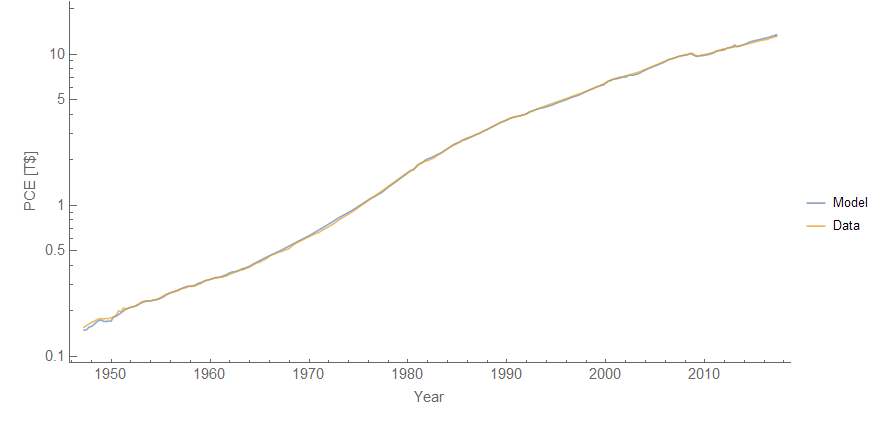

We find a = 0.82, b = 0.18, and c = -0.47. This result has several different implications. First, as John's says via Twitter, it means "consumers are way more hand to mouth than typical model[s] suggest". It also suggests that changes to income have a bigger impact on consumption than equivalent relative changes in wealth. Note that a ~ 1 means that the permanent income hypothesis isn't a good approximation (which requires a << 1) in line with previous results using information equilibrium to describe lifetime income and shocks to income. Additionally, including different methods [1] as well as John's results, the result nearly always gave a + b ≈ 1, i.e. constant returns to scale.
Overall, this is a pretty good model of consumption in terms of income and wealth.
...
Update + 3 hours
One thing to note is that the empirical finding that a + b ≈ 1 implies that there is a constant wealth-to-income ratio (for the same reasons the labor share is constant in the Solow model). This lends credence to the frequent stock-flow consistent model assumption of a constant wealth-to-income ratio (possibly subjected to stochastic shocks per the dynamic equilibrium model).
...
Update + 4.5 hours
Despite lauding John Handley above for making his code available, I forgot to upload the Mathematica code for the model to the repository (information equilibrium). This has been rectified.
Footnotes:
[1] I tried multiple different ways of estimating the parameters and all give approximately comparable results (and comparable to John's results as well).


I am not a modeller and have only skimmed the Post-Keynesian Godley & Lavoie book about stock flow consistent modelling, but what is the difference between what you are saying here and the basic consumption function introduced early in Godley & Lavoie?
ReplyDeleteGodley & Lavoie (page 66):
We suggest that households consume on the basis of two influences: their current disposable income YD, which we must assume is accurately known to households when they make their decisions,
and the wealth they have accumulated over the past, H−1. This yields
equation (3.7), which says that consumption is determined as some proportion, α1, of the flow of disposable income and some smaller proportion, α2, of the opening stock of money. Consumption functions have been subjected to intense debates, and more will be said about the relative merits and the implicit features of the one chosen here.
Cd = α1 · YD + α2 · Hh−1 0 < α2 < α1 < 1 (3.7)
Sort of ... but not quite.
DeleteThe H in the G&L model refers to government debt (change in H is G - T), but we can cede that this is household "wealth" for sake of argument. Additionally, the time step in the information equilibrium model is infinitely small.
Ignoring those pieces, then the G&L equation is an approximation to the information equilibrium equation when changes in YD or H are small.
I have to rewrite the IE relationship a bit to make this easier to understand, and I'll use G&L variables.
log(Cd/c0) = a log(YD/y0) + b log(H/h0)
The parameter c is actually a combination of c0, h0 and y0. If we take H = h0 and look at perturbations around YD = y0, we obtain (and vice versa):
Cd ~ (a c0/y0) (YD-y0)
Cd ~ (b c0/h0) (H-h0)
so we find:
α1 = a c0/y0
α2 = b c0/h0
With that "dictionary" we can relate the two equations. However, the info eq relationship also says there is an additional constant term
Cd ≈ α1 · YD + α2 · H + c0
So there are some similarities and differences.
Another difference is that there are higher order terms in the information equilibrium model:
Cd ≈ α1 · YD + α2 · H + α12 · YD² + α22 · H² + ...
One thing this model does lend credence to is the SFC idea that the wealth to income ratio is a constant. The model finds a + b ≈ 1, which means that (like in the Solow model) the two factors of production have a constant ratio (i.e. YD/H = constant) ... which is not true of the G&L model.
DeleteJason: “The H in the G&L model refers to government debt (change in H is G - T)”
DeleteYes, I should have added that the consumption equation I quoted is for the simplest SFC model (SIM) in the G&L book. The (artificial) assumption in that model is that money is the only source of wealth. Remember that the G&L book is a teaching book. The SIM model is just a way of introducing students to a basic modelling technique. The point I was trying to make was that, even at that most basic level, wealth is included in its consumption equation. If you look through the summary of notation used in the book, you’ll see that there are several other variables related to wealth which are introduced in the later (more realistic) models which relax the assumption on the composition of wealth.
The key point is that this issue is part of the ongoing debate between the Post Keynesians and the Mainstream. Irrespective of the rights and wrongs of the issue, it is not a new debate.
I put together (with a lot of help from Tom Brown) this blog post about a year back. An Alternative SIM Equation
ReplyDeleteFrankly, I have mostly forgotten the thinking behind the math but perhaps the math is simple enough that you will easily find parallels, or not.
Tom and I were tying consumption to wealth, as you seem to be doing.
Let's tie wealth, income, and consumption together. BTW, we will tie in debt as a conclusion.
ReplyDeleteLet's also look at nothing but money (for the moment) for a single time period.
Income is an increase in wealth. Consumption is a decrease in wealth. Wealth (in money) is something that accumulates over time.
So, if we consider only a one year time period, We could write the equation
Final wealth = beginning wealth plus income less consumption.
Remember, we are only including money in this equation. People also have wealth in the form of ownership of property other than money. This alternative form of wealth is not measured in income or consumption data unless it is entered as an estimated adjustment.
Now if beginning wealth is not the same as ending wealth AND we are only including money in this equation, where can the change in money-total-quantity be coming from (or going to)? If there is a change in total wealth, there must be an accompanying source or sink of the money supply itself (as a physical measurement).
The source or sink of money is debt (my argument).
(Remember--We are only including money in this equation.)
The equation as I presented it was (upon closer inspection) incorrect. The equation was incomplete in that it did not allow for new money to be created or destroyed. The complete equation should read
Final wealth = beginning wealth plus income less consumption plus newly created money
(Remember--we are only considering money in this equation.)
I think this comment shows the importance of finding a common understanding of what money really is.