Racial disparities in the unemployment rate

Unemployment by race (white = blue, black = yellow) and dynamic equilibrium (red, green).

I can't remember where I saw it on Twitter while I was on vacation, but someone graphed the most recent unemployment data by race. One of the things I noticed was the similarities in the shape of the time series. Could the disparities be explained by a single dynamic equilibrium, but with different initial conditions? Is the reason black unemployment is high today simply because it was high in the past?

It turns out the answer is basically yes.

Unlike the case of different education levels where the shape is basically the same but the dynamic equilibrium rates – the roughly constant rate of falling unemployment after a shock – are sufficiently different as to be distinguishable, the dynamic equilibrium rate for black and white unemployment is the same within model error (they are both approximately 0.09 and differ by only 0.003, see the addendum). In the graph at the top of this post, the same dynamic equilibrium fit (shown in red and green) does a reasonable job explaining both black and white unemployment (yellow and blue, respectively).

Since the model deals in logarithms, the two time series are essentially scaled versions of each other (instead of a linear model, in which they'd be shifted versions of each other). The underlying matching model is therefore the same, just with different initial conditions (higher black unemployment in 1972 than white). If white unemployment and black unemployment had been the same in 1972, then they'd be roughly the same today.

Since both white and black employment (according to this model) are hit by the same shocks, this means that black unemployment will never fall to the same level as white unemployment without some kind of intervention. Additionally, this intervention cannot be racially blind because it has to decrease black unemployment but not decrease white unemployment as much (because that would not improve the ratio). It would therefore take the form of some kind of reparations (e.g. a black-only WPA).

Addendum: Methodology

I used four different methods to apply the dynamic equilibrium model (described in detail here). I fit the entire dynamic equilibrium either to white unemployment, or black unemployment and then used that fit ‒ call it f(t), such that exp(f(t)) = u(t) with u(t) being the applicable unemployment rate  ‒ to fit to the other unemployment rate u*(t). In that second fit, I used a log-linear model:

f*(t) = f(t) + a t + b

so that u*(t) = exp(f*(t)) = exp(f(t) + a t + b). However I took a = 0 in one case (same EQ), and fit a to the data in the other. Therefore a measures the discrepancy from the dynamic equilibrium α (measuring the roughly constant logarithmic slope of the falling unemployment). The measured rates were:

Fit to white unemployment

− 0.092 = α
− 0.095 = α+a
+ 0.003 = a

Fit to black unemployment

− 0.086 = α
− 0.083 = α + a
− 0.003 = a

In both cases, black unemployment fell faster than white unemployment (i.e. the matching function performed better).

So the four scenarios/methods I looked at were:

* = black, a fit to u*(t)
* = black, a = 0
* = white, a fit to u*(t)
* = white, a = 0

The results were largely similar (within the error of the model), so I've relegated these graphs to this addendum. Here are the results (the fit data u(t) is blue, the model f(t) is red, the other unemployment data u*(t) is yellow and the other model f*(t) is green):

Dynamic equilibrium: unemployment in Hong Kong

On Twitter, John Handley brought up Hong Kong's unemployment rate as a potential counterexample/problem for the dynamic equilibrium model which says (generally) the unemployment rate will fall when not subject to a shock like a recession. In his tweets, John points out a couple of potential red flags for the dynamic equilibrium description:

Hong Kong's unemployment rate has basically been constant since 2011 

The constant increase from about 1990 to 1995 is also strange & inconsistent with constantly falling unemployment when not in recession

Now the model may not work for smaller entities like Hong Kong. However, it has roughly equivalent population to Washington State ‒ both a bit over 7 million ‒ and Washington works fine in the model. Therefore a failure would call into question at least the scope of the model, if not making us question its usefulness in general.

However, it turns out that the Hong Kong data (blue) is as well-described by the dynamic equilibrium model (red) as Washington state:

One of the key things to remember is that the normal representation of unemployment data isn't as conducive to eyeballing the success or failure of a dynamic equilibrium description. The best way to see if a dynamic equilibrium model will work is to look at a log linear transformation of the data ‒ U*(t, α) = α log U(t) + β ‒ that minimizes the entropy in the zero slope bins. For this data set, it looks like this:

The step-like appearance is the tell-tale sign of a dynamic equilibrium model. It is true that some of the steps are wider than others (corresponding to the duration of the shock); these wide shocks are what leads to the periods of approximately constant unemployment.

I did notice a feature in the HK data that appears in nearly every unemployment data set I've looked at with this model: post-recession shock overshooting. After every recession, there appears to be a brief blip of higher than expected unemployment (relative to the model). For example, here is that aforementioned WA state data:

And US data:

So there might be some other deterministic process happening along with recession shocks. It appears to be at the few percent level ‒ a potential subject for a second order model.

...

Update 29 June 2017

John Handley questioned the "just-so" nature of the shock that produced the near-constant unemployment in the most recent years. Here is the distribution of parameters for the size (amplitude) and duration of shocks for OECD countries with the recent HK shock denoted with an arrow:

Self-similarity of macro and micro

One of the things I first noticed when I started studying economics was the strange fact that the macroeconomic AD-AS model has some formal similarities to a simple microeconomic supply and demand model. In the AD-AS model, the sum of hundreds of markets for hundreds of goods behaves a bit like a single market for a single good with inflation representing the changes in price. The IS-LM model is another diagrammatic model that is formally similar supply and demand.

If you think about it, there is no real reason this has to be true. For example, DSGE models represent macro models that are not formally similar to supply and demand diagrams. Indeed, it is essentially the fallacy of composition to assume the whole works the same way as the sum of its parts. But the other interesting thing is that complex systems frequently exhibit this kind of self-similarity (just Google "self-similarity in nature" for a taste).

I was thinking about that while I was playing around with the partition function/ensemble equations for the information equilibrium model on a flight home from DC the other day. My original intent was to try to answer the question of which distribution of states preserves the scale invariance of the individual markets (so as to maybe suggest which distribution we should think about with regard to statistical equilibrium), but I ended up deriving a fascinating result.

Most of the preceding was just to set the mood. Let's dive in to a short derivation. I will start from here (which also goes into the justification of the starting point). Consider an ensemble of markets (information equilibrium relationship) $A_{i}$ with a single factor of production $B$ and IT indices $k_{i}$ so that

$$
\text{(1) }\; \frac{dA_{i}}{dB} = k_{i} \; \frac{A_{i}}{B}
$$

The solution for an individual market is

$$
A_{i} = A^{(i)}_{0} \left( \frac{B}{B_{0}} \right)^{k_{i}}
$$

Now we use the partition function $Z(B)$ to aggregate the markets. The partition function itself is:

$$
Z(B) \equiv \sum_{i} e^{-k_{i} \log B/B_{0}}
$$

Again, this is justified in the previous link. However the main point is that we assume the economy has a measurable and meaningful growth rate. If economic growth is considered to be a reasonable thing to talk about in equilibrium, then this particular approach codifies that fact in terms of a unique maximum entropy distribution.

Now let's look at some pieces we'll need. First there's the ensemble average value of $A$:

$$
\begin{align}
\langle A \rangle & = \frac{1}{Z} \sum_{i} A^{(i)}_{0} \left( \frac{B}{B_{0}} \right)^{k_{i}} e^{-k_{i} \log B/B_{0}}\\
& = \frac{1}{Z} \sum_{i} A^{(i)}_{0}\\
& \equiv \frac{\alpha}{Z}
\end{align}
$$

where $\alpha$ is defined as the sum of the coefficients $A^{(i)}_{0}$. The average IT index is

$$
\begin{align}
\langle k \rangle & = \frac{1}{Z} \sum_{i} k_{i} e^{-k_{i} \log B/B_{0}}\\
& = -\frac{1}{Z} \sum_{i} \frac{d}{d \log B/B_{0}} e^{-k_{i} \log B/B_{0}}\\
& = - \frac{B}{Z} \frac{dZ}{dB}
\end{align}
$$

Where I used the fact that $d \log B/B_{0} = dB/B$. Finally, the derivative of the average value of $A$ with respect to $B$ is:

$$
\begin{align}
\frac{d \langle A \rangle}{dB} & = \frac{d}{dB} \frac{\alpha}{Z}\\
& = -\frac{\alpha}{Z^{2}}\frac{dZ}{dB}
\end{align}
$$

Magically,

$$
\langle k \rangle \frac{\langle A \rangle}{B} = -\frac{\alpha}{Z^{2}}\frac{dZ}{dB}
$$

So we find:

$$
\text{(2) }\; \frac{d \langle A \rangle}{dB} = \langle k \rangle \frac{\langle A \rangle}{B}
$$

That is to say the ensemble average (2) is formally similar to the individual markets (1). Equation (2) is much more complex (the IT index depends on $B$), but over short periods of time where $B$ doesn't change quickly the ensemble equation can be treated as a single information equilibrium relationship.

Since you can derive a supply and demand diagram from the information equilibrium relationship (under certain assumptions), this could be seen as a short run AD-AS model. But more generally, we have a "self-similarity" in the behavior of individual micro markets and a macro ensemble of markets.

PS This basically solves something I was looking into almost exactly three years ago in these three posts: here, here and here.

PPS I'm sorry about the slowdown in posting of late. I've become much busier with work (and I'm working on a really fun R&D effort).

Barriers to entry in the quantitative parable industry

John Cochrane writes about his view of Ricardo Reis' paper defending macroeconomics. Noah Smith previously wrote about it here, and I commented on that post here. I also based my short play/Socratic dialogue in part on Reis' paper.

Cochrane provides another data point lending credence to my thesis that economists don't quite know what mathematical theory is for (see e.g. here, here, here, here, or here). The specific version that Cochrane starts off with is similar to Dani Rodrik's view (that I discuss here):

Many [critics of macroeconomics] bemoan the simplifications of economic models, not recognizing that good economic models are quantitative parables, or abstract art. Models are best when they isolate a specific mechanism in a transparent way.

Nope. 

I put the proper scientific process in picture form in this post:

Cochrane's quantitative parables go on the right hand side of this. The basic idea is that the "simple clean theoretical model" (quantitative parable, toy model) is something that comes after you've had some empirical success. In words, I'd describe the process like this:

1. Observe one or more empirical regularities [1]
2. Describe one or more empirical regularities with models (built using realistic or unrealistic assumptions ‒ your choice!)
3. Observe any errors in theoretical descriptions
4. Revise theoretical descriptions
5. Repeat/continue process
6. Collect empirical regularities and their successful models into theoretical framework
7. Test scope of theoretical framework with data, derive novel results from framework, teach the framework using toy models demonstrating framework principles, isolate mechanisms theoretically using framework for empirical study, support unrealistic assumptions using scope of the framework, and/or revise framework
8. Collect issues with theoretical framework and new empirical discoveries into new framework
9. Repeat/continue process

And this process is followed by all sciences. At any time, people can be working on steps 1 through 4. Steps 6 and 7 come along in a more mature science like physics, chemistry and biology. As far as I know, only physics has gone through step 8 multiple times (with relativity, quantum mechanics, and quantum field theory), but happy to be wrong about that. Economics has gotten to step 5 (Noah Smith has a list of some of the successes, and makes an excellent case for only getting to step 5 in this post [2]).

The key point is that the Cochrane's quantitative parables and models that theoretically isolate mechanisms come much later in the process than economics has progressed. It usually takes a genius or otherwise seminal figure to do step 6. Newton, Einstein, Noether, and Heisenberg in physics. Darwin in evolutionary biology. Hutton and Wegener in geology. Snow in epidemiology. Mendeleev in chemistry. However, we cannot use the converse: the existence of famous/seminal figures does not imply they developed a theoretical framework. And it is also important to stress the empirical piece. Wegener wasn't the first person to posit continental drift, but was the first to include e.g. fossil evidence. Economics in contrast is rife with theoretical frameworks posited by famous economists without comparison to empirical data. Even Keynes and Adam Smith appeal to philosophy and argument rather than data ‒ Keynes famously saying "But it is of the essence of a model that one does not fill in real values for the variable functions."

As an aside, I think I might have finally arrived at a really good way to describe what critics are saying when they say economists have "physics envy": economists think they have a theoretical framework. It explains why economists have papers with overly-mathematical symbols given how poorly the theory describes the data. It explains why they feel they can make unrealistic assumptions even when the result doesn't describe any data. It explains why they think the words "toy model" should even be in their vocabulary. Economists think they are in step 7, but really they are still cycling through step 5.

That seems like a bad start for Cochrane's piece, but the next thing he says is right on:

Critics [of macroeconomics] usually conclude that we need to add the author's favorite ingredients ‒ psychology, sociology, autonomous agent models, heterogeneity, learning behavior, irrational expectations, and on and on ‒ stir the big pot, and somehow great insights will surely come.

There is far too much "we should include X" in economics (including heterodox and non-economists). The only scientific way to say "we should include X" is to say:

APPROPRIATE: We included X and it improved the theoretical description of empirical data, therefore we should include X.

The unfortunate thing that some scientists do however is this:

INAPPROPRIATE: "We included X and it improved the theoretical description of empirical data in our field of science, therefore we should include X in economics.

It would be fine if it improved the theoretical description of empirical data in economics, but theory by analogy only goes so far. I try to call this out as much as possible when I can (biology, evolutionary biology, complexity theory).

I think this is the unfortunate consequence of the history of theoretical frameworks without reference to empirical data in economics. If you don't discipline theory in your field with data, anyone thinks they can come up with a theory because they reckon they know a bit about how humans think about money being a human who has thought about money.

And that's really a bigger takeaway. Many macroeconomists are frustrated with the criticism and the economic ideas coming from people without PhDs in economics. But they set up their field to essentially be armchair mathematical philosophy, and the barriers to entry for armchair mathematical philosophy are extremely low. A high school education is probably more than sufficient. I think that explains the existence of the econoblogosphere. It's really not the same in physics, mathematics, or signal processing from my experience (using examples of my favorites) ‒ those fields all tend to have experts and PhD students sharing ideas.

I think I'll leave it there because this forms a nice single thesis. There is a process to science and mathematical theory has a specific place. However, theory without comparison data or without an empirically successful framework is just armchair mathematical philosophy. There are few barriers to entry in armchair philosophy. For toy models isolating mechanisms however, empirical success is the barrier to entry. 

...

PS I did get a chuckle out of this:

Others bemoan "too much math" in economics, a feeling that seldom comes from people who understand the math.

I think that is sometimes true. 

However, I personally do understand the math. My opinion is that 1) the level of mathematical complexity of macroeconomic models far outstrips the limited amount of empirical data, and 2) the level of mathematical rigor far outstrips the accuracy of those models.

PPS I imagine some people will call me out for hypocrisy regarding the "INAPPROPRIATE" statement above. Aren't you, physicist, saying things from physics should be included in macroeconomic theories?

I would remind those people that I am not forgetting the clause about comparing to empirical data. I am not saying just "economists should use information theory", I am saying the information theory nicely encapsulates several empirical successes. I also test the theory with forecasts.

...

Footnotes:

[1] Yes, you always need to have some sort of underlying model in order to collect and understand data. However this is not that onerous of a requirement as even philosophy can frequently fill this role. An example is Hume's uniformity of nature. The implicit model behind the unemployment rate is that there are some people who do things in exchange for money and some people looking for opportunities to do things in exchange for money. 

Sometimes people make this observation out to be much more consequential than it actually is. Sure, it's important in the case of understanding what fluctuations of NGDP are important (i.e. what is a recession). However a lot of empirical data in economics is "counting things" where the implicit theory is not much more complex than the one that governs "Which recycling bin does this go in?"

[2] Added 4pm. In contrast to Noah's opinion, though, I wouldn't say that makes economics "not quite" science. It's true that most of the "hard" sciences made it to step 7, but they once were in steps 1 through 4. Physics didn't suddenly become "science" after Newton. It just became a science with a theoretical framework. Biology didn't become a science after Darwin, it was just more about empirical data before.

I think macroeconomics and microeconomics prematurely thought it had a framework with rational utility maximization and some ideas from Keynes (the neoclassical synthesis). Economists started to evade the discipline of data. In a sense, what Noah is calling the "credibility revolution" is the slow realization that the purported frameworks like rational utility maximization and DSGE failed some of the tests in step 7 and so macro is falling back to steps 1-4. This is a good development.

Forecast stability (unemployment rate edition)

I have an old post where I proposed a though experiment: What would the charts of economic forecasts look like over time if they were made with the incorrect model?

Well, the FRBSF has revised their unemployment rate forecast once again in the latest issue of FedViews so I went back and compiled their forecasts from the beginning of 2015, 2016, and 2017 (shown in different colors below) into a single chart reminiscent of the thought experiment charts. Basically, the FRBSF has continued to revise their forecast for the unemployment rate downward over time.

In addition to compiling those forecasts, I made forecasts using the dynamic equilibrium model (gray) from the same starting date as the FRBSF forecasts (shown with a vertical gray line).

Here are the results:

While, yes, the dynamic equilibrium model does pretty well in terms of residuals, I wanted to bring attention to another desirable quality of models: the dynamic equilibrium forecasts are relatively stable with respect to incoming data (and in fact converge over time).

Now it is true that the unemployment rate will almost inevitably go up again at some point in a future recession. And recessions do introduce some instability into the dynamic equilibrium forecasts of the unemployment rate (as you can see in the algorithmic recession detector), but that instability occurs exactly where we should tolerate it more: a dynamic non-equilibrium situation like a recession. The FRBSF instability occurs during what we'd otherwise consider a "normal" economy.

Information transfer economics FAQ (reference post)

FAQ (Frequently Asked Question) pages used to be a more prevalent aspect of the internet, but seem to be fading ‒ probably due to being able to ask those questions directly in a Google search or on Quora or similar sites. Anyway, this will be a reference post that will be occasionally updated with some of the questions and misunderstandings I frequently run across from readers. Here's a link to some basic definitions that I'll assume readers have read.

Don't economists already study information in economics?

The "information" in information transfer economics is from information theory and the study of communication channels. It has a technical definition more directly related to probability than to e.g. knowledge of how the monetary system works or whether a company is about to announce disappointing earnings. The key insight from Shannon in his seminal paper on the subject was that the meaning of messages sent through a communication channel is not as important as the number of possible messages (which determines the information content of each message). It's that state space that matters here.

That being said, the work of Christopher Sims comes closest to treating information in a similar way. (And he finds the message doesn't seem matter!)

Why do you treat economic agents as mindless atoms?

This is a bit of a mischaracterization of how the information equilibrium/dynamic equilibrium framework treats economic agents. The best way to put it is that the framework treats humans as so complex their decisions appears to be algorithmically random (i.e. indistinguishable from a computer program with random outputs for a given set of inputs). The main assumption however is that an ensemble of economic agents will fully explore the possible options available to them in the presence of constraints. The net result is a model that looks like "mindless atoms", but it isn't the whole story. 

This approach is somewhat different from traditional economics where agents are usually assumed to choose the best option available to them. However, economist Gary Becker had a paper from 1962 that also looked at this "random" approach (thanks to economist David Glasner to pointing it out to me). He [Becker] referred to it as "irrational", but I am agnostic as to the motivations of the agents. Even a rational decision can look like an irrational one if you are missing some knowledge of the agent (e.g. selling a stock at a loss in recession looks irrational, but it is possible the person had medical bills to pay).

But mindless atoms don't panic ...

While information equilibrium treats agents effectively as random "mindless atoms" (but really treats them as so complex they look random), the information transfer framework is more general. If agents didn't spontaneously correlate in state space due to human behavior (e.g. panic, groupthink), then the information transfer framework reduces to something that looks like boring standard thermodynamics. However, they do in fact panic. In terms of thermodynamics, this means that the information transfer framework is like thermodynamic, but missing a second law of thermodynamics. The "mindless atoms" will occasionally panic and huddle in a corner of the room and you have non-ideal information transfer as opposed to information equilibrium.

There is less the information transfer framework can say about scenarios where we have non-ideal information transfer, but it still could be used to put bounds on economic variables.

Wait. Isn't this just saying sometimes your theory applies and sometimes it doesn't?

Yes, but in a particular way. For example, the effect of correlations (panic, groupthink) is generally negative on prices.

Additionally, empirical data appears to show that information equilibrium is a decent description of macroeconomic variables except for a sparse subset (i.e. most of the time). That sparse subset seems to correspond to recessions. Since human behavior is one of the ways the system can fail to be in information equilibrium, this is good evidence that information equilibrium fails in exactly the way the more general information transfer framework says it should.

In a very deep way, one can think of information equilibrium being a good approximation in the same way the Efficient Market Hypothesis (EMH) is sometimes a good approximation. Failures of the EMH seem to be correlations due to human behavior.

If your theory is so awesome, why aren't you well known in economics circles?

The short answer is: I don't know. You'd think forecasting better than macro institutions would somehow get out there more. But I think the bulk of  econ twitter and the dwindling econoblogosphere is more interested in how they think the economy works than how it actually works.

That said, I was invited to give a talk at my local university's (and alma mater's) economics department — so I'm guessing like most things in academic research it's more of a long slog than becoming a rock star overnight.

Well, why haven't you at least been published then?

It's apparently really hard to be published in an econ journal even if you're a famous professor, with revisions often taking years. If you don't have an econ degree, you're almost certainly going to get desk rejections (as I have).

I have two papers (so far) available as pre-prints (here and here) and at least in physics and machine learning these are basically the only things people read these days because publishing is so slow. Even economics does basically the same thing, except their pre-print server is closed off to everyone except insiders.

Why don't you get rich using your theory?

In a way, I am because my 401(k) is invested in index funds. The theory says that unless you can predict human behavior, you cannot predict episodes of non-ideal information transfer. Therefore the optimal portfolio choice is to diversify and hold for a long period of time. This is what most financial advisers say anyway (and the reason is effectively the same: because the EMH is a good starting approximation).

Some individual people might well be good at predicting human behavior and therefore could potentially outperform the diversified index fund investor, but I am not one of those people. Individual human behaviors frequently baffle me.

I have put together some speculative research about stock markets, but again the results are broadly similar to already known investment strategies.

So you have economics all figured out?

No, not in the slightest. This is all research. I am currently testing the models using empirical data and forecasts. Readers should not confuse my excitement and interest for certainty.

Are you a heterodox economist?

Not really because heterodox econ is its own thing. Though I have no issues with any approach that is honest in its representation — especially because economics is at best a nascent science.

But you're definitely saying mainstream economics is wrong?

Not really. I do believe there are some assumptions made in many (mainstream and heterodox) approaches in economics about the impact of human decision-making, human behavior, and complexity of the macroeconomic system that are unfounded from an empirical perspective. A simpler approach like information equilibrium avoids making strong assumptions about human behavior (we only assume agents explore opportunities most of the time) and uses information theory as a shortcut to understanding complex systems (per the abstract of Fielitz and Borchardt's original paper on information equilibrium for natural systems).

That being said, information equilibrium can be used to formulate many mainstream economic models. Several of these information equilibrium versions of mainstream models tend to be less empirically accurate than information equilibrium models constructed from observed empirical regularities directly (a good example is the New Keynesian DSGE model versus the monetary information equilibrium model).

In the sense that modern economics grew out of the principles of supply and demand and marginalism, one can think of information equilibrium/information transfer as a generalization of those principles. It therefore has some overlap with mainstream economics.

Have you heard of Duncan Foley?

Yes.

Have you heard of Steve Keen?

Unfortunately, yes.

What about MMT?

*sigh*

But how could you possibly find anything wrong with MMT?

*eyes roll back in head*

But what about X?

Over the past six years (as of 2019), I have written over a million words on information equilibrium, dynamic equilibrium, information transfer, and the applications to economics. I probably have written about X, so have a look via the search bar (or better yet a Google site search like this for "scope" which will search comments as well). I try to use mainstream economics terminology where I can, so you can use phrases like nominal rigidity or tâtonnement. Comments are open on all of the older posts if you have questions.

If you're looking for a good place to start, I put together a "tour of information equilibrium" chart package.

Wasserstein GAN and information equilibrium

A figure from Arjovsky, Chintala, and Bottou showing the lack of a strong gradient in the Jensen-Shannon divergence, slightly edited for comedic effect.

This paper (Arjovsky, Chintala, and Bottou [ACB]) on Wasserstein Generative Adversarial Networks (WGANs) has been generating (no pun intended) a lot of buzz in the machine learning community. Earlier this year, I mentioned some intuition I had about a possible connection between GANs and information equilibrium as well as the potential for GANs to function as a model of markets.

ACB uses the Wasserstein distance (metric) (also called the Earth Mover's Distance) instead of the original Jensen-Shannon distance (divergence) (a symmetric version of the Kullback-Liebler divergence). One of the benefits of the W-metric for machine learning is that it tends to have non-zero gradients (so e.g. gradient descent solvers won't have as many issues as could happen with other metrics illustrated in the figure at the top of this post). In an odd coincidence, the W-metric has come up two other times recently in unrelated contexts in my real job.

I noticed that this approach also has some interesting connections to information equilibrium. For starters, the W-metric is very much the intuitive guide I usually give for the distribution of supply coming into equilibrium with demand. We have two distributions where a lump of the supply distribution is moved to some place where there is an excess in the demand distribution as part of our approach to equilibrium. Here's a figure illustrating the concept from a nice discussion of WGAN:

There is even a happy accident in terminology in that there is a "cost function" involved. There is an additional happy accident that the exact solution for histogram distributions is obtained via linear programming, discussed in the context of economics in this blog post. By the way, there is an another nice overview of ACB here.

One of the other interesting aspects of WGANs is that the GAN "discriminator" is replaced by a WGAN "critic" (per ACB via the previous link):

The critic makes much more sense in the context of economics: at constant demand, a low price is a "critic" of excess supply and a high price is a "critic" of scarce supply.

The GAN analogy is still a one-sided model of supply and demand (it is a model for constant demand and varying supply or vice versa), rather than a full "general equilibrium" analogy (where supply and demand react to changes in each other).

I'm going to close (for now) with another observation about some of the math involved, namely Lipschitz functions. One of the problems with the abstract WGANs is that the W-metric is generally intractable (like the linear programming economic allocation problem). However one can rewrite the problem using Kantorovich-Rubinstein duality which couches it in terms of Lipschitz functions which are (put simply) functions with bounded slope. The K-Lipshitz condition (bounded by slope K) is:

d​ₙ​​​(f(m​₁​​), f(m​₂​​)) ≤ K dₘ​​(m₁​​, m​₂​​)

for all

m₁ and m​₂ 

where f(m) : m → n and the d's are metrics on the manifolds m and n. Longtime readers of this blog may know where this is going already: this can be represented as an information equilibrium (transfer) condition. If we have information transfer from "demand" A to "supply" B, then:

dA/A ≤ k dB/B

d(log A) ≤ k d(log B)

which is the infinitesimal version of the K-Lipschitz condition (for log A and log B) with the IT index k playing the role of the slope K. That is to say that information transfer relationships are "locally" k-Lipschitz. The definition of K-Lipschitz is actually a global (i.e. for all of m (i.e. log B)), so the KR duality trick would only work functions that are in information equilibrium (i.e. the equal sign, because then log A = k log B + c and the slope is actually equal to k for all log B measured from any two points log b₁ and log b₂).

[Update 19 June 2017: n.b. this also applies to the price p = dA/dB being locally K-Lipschitz, but with K = k − 1.]

The Lipschitz function representation of the WGAN also yields a solution up to an overall scale. I discuss the potential importance of scale invariance in economics in several posts (e.g. here or here).

I am not sure there is anything useful in the observation; it may be wildly off-base. I am still looking into the possible use of of GANs as a model of the "market algorithm", possibly showing us how markets work as well as under what conditions they don't work (and ways to improve them).

Today's Fed decision and recession indicators

The Fed makes its interest rate announcement today at 2pm Eastern (11am Pacific). If they raise rates, then a couple of recession indicators will move towards the higher probability of recession end of the spectrum. For example, there's the inverted yield curve (discussed more extensively here):

There is also the "avalanche" indicator (the yellow area indicates above-trend interest rates and recessions never seem to happen without them):

Additionally, several of the JOLTS measures are showing a slowdown relative to the dynamic equilibrium (in this graph, the hires data is starting to fall below the green line):

Up until the last couple data points, the unemployment rate was seeming to flatten out signalling a potential recession in the dynamic equilibrium model:

All of this is of course speculative, with only the inverted yield curve being a mainstream indicator. However, if the information equilibrium/dynamic equilibrium picture is correct, we are starting to accumulate several indicators of a future recession. Each on its own is definitely not enough, and the Fed could hold off raising rates today due to a low CPI inflation number (making yield curve less likely):

However, I wanted to get this out there before the Fed announcement today to both make sure I'm keeping myself honest as well as providing a test of the usefulness of the information equilibrium model.

...

Update 11:32am

They raised them.

Consumption, income, and wealth

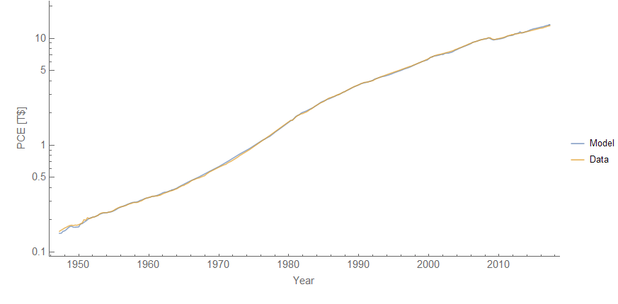
John Handley has started up a new updated blog, and the most recent post asks an interesting question (in a way that should be lauded for both its use of data and making the code available): if disposable income predicts consumption so well (i.e. the traditional Keynesian consumption function), why did anyone start using the Euler equation with its "almost comical level of inaccuracy"? While we wait for the optimal answer to that question from Beatrice Cherrier, my intuition says the answer is "microfoundations". John asked me to verify his regressions, which I did; the model he considered has the added benefit of being an information equilibrium model so I am writing it down here.

The basic Keynesian consumption function is essentially a linear model

PCE = a DPI + c

where PCE is personal consumption (FRED PCEC) and DPI is disposable income (FRED DPI). However John discovered an excellent relationship between PCE, DPI and total net worth (FRED TNWBSHNO) which I will call TNW for short:

log PCE = a log DPI + b log TNW + c

This has the form of an information equilibrium relationship (as well as a Cobb-Douglas production function where income and wealth are both "factors of production" for consumption):

PCE ⇄ DPI

PCE ⇄ TNW

with information transfer indices a and b. It also reduces to the basic Keynesian model in the limit where changes in TNW and DPI are small (in percentage terms). The model works pretty well [1]:

We find a = 0.82, b = 0.18, and c = -0.47. This result has several different implications. First, as John's says via Twitter, it means "consumers are way more hand to mouth than typical model[s] suggest". It also suggests that changes to income have a bigger impact on consumption than equivalent relative changes in wealth. Note that a ~ 1 means that the permanent income hypothesis isn't a good approximation (which requires a << 1) in line with previous results using information equilibrium to describe lifetime income and shocks to income. Additionally, including different methods [1] as well as John's results, the result nearly always gave a + b ≈ 1, i.e. constant returns to scale.

Overall, this is a pretty good model of consumption in terms of income and wealth.

...

Update + 3 hours

One thing to note is that the empirical finding that a + b ≈ 1 implies that there is a constant wealth-to-income ratio (for the same reasons the labor share is constant in the Solow model). This lends credence to the frequent stock-flow consistent model assumption of a constant wealth-to-income ratio (possibly subjected to stochastic shocks per the dynamic equilibrium model).

...

Update + 4.5 hours

Despite lauding John Handley above for making his code available, I forgot to upload the Mathematica code for the model to the repository (information equilibrium). This has been rectified.

...

Footnotes:

[1] I tried multiple different ways of estimating the parameters and all give approximately comparable results (and comparable to John's results as well).

Milton Friedman's question begging

Nick Rowe tweeted his post about "Milton Friedman's thermostat" where he begins:

I know I'm right in saying that Milton Friedman's thermostat is an important idea that all economists ought to be aware of. And I'm pretty sure I'm right in asserting that almost all economists are unaware of this important idea that all economists ought to be aware of.

If Nick is right about economists being unaware of it, then there's a good reason: it's not a logically valid argument.

Nick retells Friedman's parable using a gas pedal g(t) and a car's speed s(t) going up and down hills h(t). The basic premise is that if the driver perfectly achieves a target speed of 100 km/hr, then it will look like the gas pedal movements are unrelated to speed (if we don't know about the hills). The gas will be going up and down, but the speed will be constant.

The argument purportedly can be deployed at anyone using data to claim the gas pedal doesn't matter.

But how did either the plaintiff or the defense know the gas pedal had anything to do with this scenario in the first place? Friedman's thermostat assumes some prior empirically validated model where the gas pedal was conclusively proven to determine the car's speed before the "constant speed" scenario came to be.

That is to say a scientist just given the "constant speed" scenario would say there's no evidence anything influences speed. The "best model" is actually a constant

s(t) = 100 km/hr

Not

s = s(h(t), g(t), t)

If you already know g(t) matters ‒ and adaptively makes s(t) constant ‒ then, yes, the constant s(t) data doesn't disprove that. But if it is a question whether g(t) matters, then assuming g(t) matters in order to disprove claims that g(t) doesn't matter is classic question begging.

Additionally, in order to disprove claims that g(t) doesn't matter one could just deploy the original data and findings that g(t) does matter. This of course makes Friedman's thermostat superfluous.

So hopefully that's why most economists don't know about Milton Friedman's question begging, I mean, thermostat.

Now it is true that when Friedman deployed the argument [pdf], he said there was a time when the thermostat was imperfect before the analog of the "constant speed" scenario ‒ which allows one to determine the effects of g(t). However it is not an undisputed fact that g(t) was determined to affect speed (for example, post war inflation is arguably a demographic effect).

At the end of the day, it's usually best to argue about models in terms of empirical data rather than logic and philosophy.