The Phillips curve

Earlier this year John Quiggin made the bold claim that macroeconomics went wrong in 1958 after the discovery of the Phillips curve. I've been working over the past couple months trying to figure out how the Phillips curve comes about in the information transfer framework and I basically come to the same conclusion. Here is my bold claim:

The Phillips curve is real but barely useful regularity in the data that has been completely misinterpreted.

OK, let's begin. The curve is generally drawn as a downward sloping curve in unemployment rate-inflation rate space. In the information transfer model, this immediately says that the information source is aggregate demand (NGDP), the information destination is the supply of unemployed people (U, e.g. this metric -- and n.b. here and throughout U is the total number of unemployed, not the unemployment rate), and the price level P is detecting signals from the demand to the supply. In my notation, P:NGDP→U. Therefore we can write 

$$
\text{(1) } P = \frac{1}{\kappa} \frac{NGDP}{U}
$$

We can do a fit to the data (price level in green, model in blue)

This fit works as well as the fit to the interest rate in the IS-LM model, so it gives some hint that we may be able to extract information from it. One interesting thing to consider is that the price level curve could define a "natural rate" of unemployment (actually more of a mean level of unemployment, blue):

The graph divides the number of unemployed by the size of the civilian labor force (L) to get the unemployment rate. Here is the graph of deviations from the blue curve:

I've excised the recessions in the data points (dots) in the graph above. It becomes clear that most of the data points and nearly all of the non-recession data points represent an unemployment rate that is falling. This is a major point in understanding the Phillips curve in the information transfer framework. Of course, to get to our final destination requires a little math. Start with the price level equation (1) above and take the logarithmic derivative:
$$
\frac{d}{dt} \log P = \frac{d}{dt}\log \frac{1}{\kappa} \frac{NGDP}{U}
$$
Expanding that out a little
$$
\frac{d}{dt} \log P = \frac{d}{dt}\log NGDP -\frac{d}{dt}\log U -\frac{d}{dt}\log \kappa
$$
Identifying the inflation rate $\pi$ (borrowing from the notation in the wikipedia entry) and the NGDP growth rate $n$, and taking $\kappa$ to be constant ($\simeq 0.6$ by the way), and fiddling with the $U$ term:
$$
\pi = n -\frac{1}{U}\frac{d}{dt}U
$$

If we expand around the number of unemployed at natural rate $U^*$ (or really any fixed level of unemployed rate) and taking $dU/dt = U'$ we can write:

$$
\pi = n -\frac{U'}{U^*} + \frac{U'}{U^{*2}}(U-U^*)
$$

Or in terms of the unemployment rate $u = U/L$ where $L$ is the civilian labor force:

$$
\pi = n -\frac{U'}{U^*} + \frac{U' L}{U^{*2}}(u-u^*)
$$

Where we make the notational identifications $n -U'/U^* = \pi^e + \nu$ and $B = U' L/U^{*2}$ we finally obtain the new classical form of the Phillips curve:

$$
\pi = \pi^e + \nu + B (u-u^*)
$$

... except there's a problem: the sign of the $B$ term is "wrong". This is where the observation in the previous graph comes in. Nearly all the data has $U' \lt 0$ so in most descriptions of the data we can take $b = |U' L/U^{*2}|$ positive and write

$$
\pi = \pi^e + \nu - b (u-u^*)
$$

The regularities of the Phillips curve essentially result from the fact that recessions tend to cause unemployment to shoot up quickly and then drift back down slowly over a longer period. With this knowledge we can see what the data looks like when excluding data where $U' > 0$:

Graphs of the Phillips curve tend to be broken up into "regimes" (from the wikipedia article we have 1955-1971, 1974-1984, 1985-1992 and 2000-2013); we can see how this segmentation approximates the behavior of the parameters $b$ and $\pi^e + \nu$:

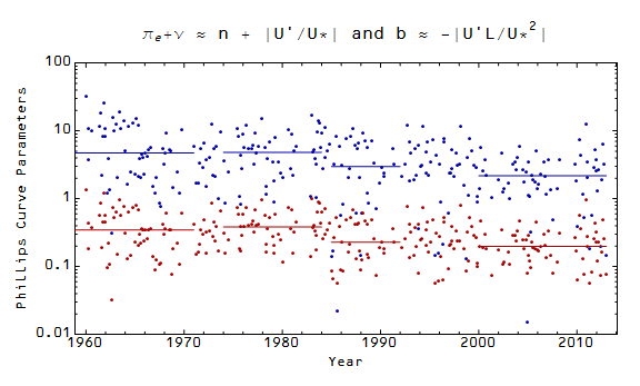
Basically, the Phillips curve "regimes" represent relatively constant segments of the parameter values. Here are the graphs of the resulting Phillips curves for the different "regimes":

This allows us to posit a reason for the failure to find microfoundations for the Phillips curve. It is a property of the unemployment rate (quick rise, slow fall) that is only marginally connected to inflation (the slow fall in unemployment occurs during a recovery hence during a temporary increase of the inflation rate from a low level brought on by the recession). The real nugget of statistical regularity is that a recession causes unemployment to rise and inflation to fall with the Phillips curve describing the subsequent return to normal (unemployment to fall and inflation to rise). Or another way, the Phillips curve is just mean reversion. And mean reversion doesn't really need microfoundations, does it?

In any case, the Phillips curve is dependent on the dominance of data where $dU/dt < 0$ after recessions.