Saturday, June 25, 2016

About that graph ...

There's a graph I've seen around the internet (most recently from Timothy B. Lee on Twitter) that contains the message: "The earlier you abandon the gold standard and start your new deal, the better ..." typed over a graph from Eichengreen (1992):


Looks pretty cut and dried, but I'd never looked at the data myself. So I thought I'd have a go at figuring out what this graph looks like outside of the domain shown. First note that this is a graph of an industrial production index, not NGDP, normalized to 1929. The data was a bit difficult to extract; some is just from FRED, others digitized from the graph itself and a few extra points from Japan come from this interesting article from the BoJ [pdf] about economy during this time period. The results make the case a little less cut and dried (colors roughly correspond):


The graph at the top of this post is shown as the gray dashed line. First, with the other data, it is hard to say anything much is happening in the UK:


The UK actually pegs its interest rate at 2% in the period of the gray bar (which seems to generate inflation), but the overall picture is "meh". However, in that article above, we learn Japan actually started a "three-arrow" approach (similar to the one employed in Abenomics) in 1931 that included pegging its currency to the UK (gray bar in graph below):


Now pegging your currency to another is abandoning the gold standard (at least if the other currency isn't on the gold standard, which the UK didn't leave until later according to the graph -- when it also started pegging its interest rate). Additionally, in 1931, Japan's military build up that would eventually culminate in the Pacific theater of WWII began (remember, this is an industrial production index). Military build up (starting in 1933) and pegged interest rates (gray) could be involved in Germany as well:


We can pretty much leave France out of the conclusion of the graph at the top of the page because there's really no data. That leaves the US:


The pegged interest rates (gray) don't seem to have much to do with the highlighted red segment (see more here about the US in the Great Depression and the Veterans bonus; see also here and here about the period of hyperinflation and price controls), but the New Deal, started in 1933 probably does. It could be the gold standard, but having both happen at the same time makes it hard to extract the exact cause. In fact, you could even say this is just a relatively flat random walk from 1920 until the US military build-up starts in 1939. Without WWII, I could have seen this graph continuing to the right with periods of rising and falling industrial production.

So what looks like a cut and dried case about the gold standard may have much more to do with fiscal policy than monetary policy. In fact, what seemed to happen was that bunch of different policies were tried and we still can't quite extract which one did what -- the answer is likely a muddle of fiscal and monetary policies. And we haven't even gotten to whether industrial production is the right metric.

Friday, June 24, 2016

Gronwall's inequality and information transfer


In light of Brexit, non-ideal information transfer is now much more salient. And because of that, I thought it might be a good time to post this information transfer-specific form of Gronwall's inequality that's been languishing as a draft for awhile.

...

One of the key lemmas I've used liberally to say the solution of a differential inequality is bounded by the solution of the corresponding  differential equation is called Gronwall's inequality. It's useful in stochastic differential equations, among other applications. It is not a general result for all differential equations, but fortunately applies precisely in the case we consider in the information transfer framework. It is written differently in the Wikipedia article linked, but I'd like to show this is just a notational difference. The differential equation that the inequality applies to is 

$$
u'(t) \leq \beta (t) u(t)
$$

This is just the equation

$$
\frac{du(t)}{dt} \leq \beta(t) u(t)
$$

and if $\beta (t) = k/t$, we have

$$
\frac{du(t)}{dt} \leq k \; \frac{u(t)}{t}
$$

and we can select the variables to be whatever we'd like (and take the function arguments to be implied). Therefore, given an information transfer relationship $\alpha \rightarrow \beta$, we can say the solution to the differential inequality:

$$
\frac{d\alpha}{d\beta} \leq k \; \frac{\alpha}{\beta}
$$

is bounded by the corresponding information equilibrium relationship $A \rightleftarrows B$

$$
\frac{dA}{dB} = k \; \frac{A}{B}
$$

with solution

$$
A(B) = A(B_{ref}) \exp \left( k \int_{B_{ref}}^{B} dB' \; f(B') \right)
$$

taking $A(B_{ref}) \equiv A_{ref}$ and integrating $f(B') = 1/B'$

$$
A(B) = A_{ref} \exp k \left( \log B - \log B_{ref} \right)
$$

rearranging (and putting it in the form I usually use)

$$
\frac{A}{A_{ref}} =  \left( \frac{B}{B_{ref}} \right)^{k}
$$

Therefore

$$
\frac{\alpha}{\alpha_{ref}} \leq  \left( \frac{\beta}{\beta_{ref}} \right)^{k}
$$

i.e.

$$
\alpha(\beta) \leq \alpha(\beta_{ref}) \exp \left( k \int_{\beta_{ref}}^{\beta} d\beta' \; f(\beta') \right)
$$

Thursday, June 23, 2016

Summer blogging recess (and no-go theorems)

I have a bunch of things to attend to over the next month or so, so there will be few (if any) posts. I plan on working (the real job), taking a couple of trips (work- and non-work-related), thinking about a problem Cameron Murray suggested, and finishing up the first draft of the book (see here; I've been spending some time away from the draft, hoping to come back to it with new eyes).

I will also continue to be baffled by the stock-flow accounting advocates (see comments here and here). It seems more and more to be a paradigm akin to market monetarism to me. Market monetarism exists in order to deny the effectiveness of fiscal stimulus [as a primary policy tool]; Stock-flow accounting exists to deny the existence of any weakly-emergent properties of macroeconomies. Everything they seem to say is inconsistent with this picture:


Not this model, mind you, but the existence of this picture. The weakly-emergent travelling wave cannot exist -- even though this kind of weakly-emergent structure is perfectly consistent with strict accounting of the variables.

All I get in response are attempts to teach me accounting! Trust me -- accounting "theorems" don't quite rise to the level of Stokes' Theorem; this stuff is not complex except in vocabulary. I have degree in math with particular emphasis in topology and differential geometry. The discrete point set on which accounting is defined can't be more complex that the typical topology of the Cantor set. However, the main issue is that "you don't understand accounting" isn't particularly responsive to the question: Why are there no weakly-emergent (e.g. field) quantities in systems that obey accounting principles?

Is there some proof of this? It would be some kind of no-go theorem for certain covering spaces of a space defined by a set of functions on some discrete point set, network, or connected intervals. This is of course not generally true: all of solid state electronics is a counterexample, as well as things like temperature and pressure.

There would have to be something specific about the accounting equations that prevents this. However, accounting operators aren't exactly elliptic differential operators, so I have difficulty imagining a no-go theorem arising from addition and multiplication.

This may sound like I' trying to win an argument by bringing up a lot of high level mathematics, but that's actually what's at issue. Denying weakly emergent quantities is a pretty high level mathematical question about the properties of discrete spaces. I can't imagine it can be answered by double entry bookkeeping.

Monday, June 20, 2016

Metzler diagrams from information equilibrium


Paul Krugman has a post today where he organizes some DSGE model results in a simplified Mundell-Fleming model represented as a Metzler diagram. Let me show you how this can be represented as an information equilibrium (IE) model.

We have interest rates $r_{1}, r_{2}$ in two countries coupled through an exchange rate $e$. Define the interest rate $r_{i}$ to be in information equilibrium with the price of money $M_{i}$ in the respective country (with money demand $D_{i}$) -- this sets up four IE relationships:

$$
\begin{align}
r_{1}&  \rightleftarrows p_{1}\\
p_{1} :  D_{1}& \rightleftarrows M_{1}\\
 r_{2}& \rightleftarrows p_{2}\\
p_{2} :  D_{2}& \rightleftarrows M_{2}
\end{align}
$$

This leads to the formulas (see the paper)

$$
\text{(1) }\; r_{i} = \left( k_{i} \frac{D_{i}}{M_{i}}\right)^{c_{i}}
$$

Additionally, exchange rates are basically given as a ratio of the price of money in one country to another:

$$
e \equiv \frac{p_{1}}{p_{2}} = \alpha \frac{M_{1}^{k_{1}-1}}{M_{2}^{k_{2}-1}}
$$

And now we can plot the formula (1) versus $M_{1}^{k_{1}-1}$ (blue) and $M_{2}^{1-k_{2}}$ (yellow) at constant $D_{i}$ (partial equilibrium: assuming demand changes slowly compared to moneytary policy changes). This gives us the Metzler diagram from Krugman's post and everything that goes along with it:


Also, for $k \approx 1$ (liquidity trap conditions), these curves flatten out:


Stock flow accounting with calculus


Commenter Peiya took issue with my comments on stock-flow analysis in the previous post. This post is mostly a response to point (3) that needed a bit more space and mathjax to be properly addressed.

The equation in question is (call stock $S$ and flow $F$, and define a revaluation functional $\alpha = \alpha [S]$):

$$
S(t) = \alpha [ S(t-\Delta t) ] + F(t)
$$

First, let's say $S(t-\Delta t) = 0$ (you're starting from zero), then this equation asserts $S(t) = F(t)$, i..e stock is equal to a flow. This doesn't make sense unit-wise (a flow represents a change in something and therefore has to happen over a period of time, hence there is a time scale associated with the right hand side, but not the left). Per Peiya, $F(t)$ is defined on an interval $[t, t + \Delta t)$, this allows us to define a function $\phi$ (assuming $F \in C^{2}$ except on a countable subset) with the same support such that

$$
F(t) \equiv \int_{t}^{t + \Delta t} dt' \phi(t') = \Phi (t+\Delta t) - \Phi (t) \equiv \Delta \Phi
$$

Thus we can actually see that $F$ is really a stock variable made from a change in stock over some time scale. Assuming a short interval where $\phi$ is approximately constant, we can see the time scale $\Delta t$ pop out:

$$
F(t) \approx \int_{t}^{t + \Delta t} dt' \phi \approx \phi \cdot \Delta t \equiv \Delta \Phi
$$

So how do we treat stock-flow analysis in a way that is consistent with mathematics? Let's start from $t = 0$ in that first equation. We have (taking a constant revaluation $\alpha$ per time period for simplicity, but can be handled in the general case as long as $\alpha$ isn't pathological)

$$
S(\Delta t) = \int_{0}^{\Delta t} dt' \phi_{1}(t')
$$

$$
S(2 \Delta t) = \alpha \int_{0}^{\Delta t} dt' \phi_{1}(t') + \int_{\Delta t}^{2\Delta t} dt' \phi_{2}(t')
$$

$$
S(3 \Delta t) = \alpha^{2} \int_{0}^{\Delta t} dt' \phi_{1}(t') + \alpha \int_{\Delta t}^{2\Delta t} dt' \phi_{2}(t') + \int_{2\Delta t}^{3\Delta t} dt' \phi_{3}(t')
$$

etc, so that (taking $\phi_{k} = 0$ outside the interval $[(k-1) \Delta t, k \Delta t)$, we can write

$$
S(t = n \Delta t) = \int_{0}^{t} dt' \sum_{i = 1}^{n} \alpha^{i-n} \phi_{i}(t')
$$

and defining

$$
\sum_{i = 1}^{n} \alpha^{i-n} \phi_{i}(t') \equiv \tilde{\phi} (t')
$$

we obtain (assuming $S \in C^{2}$ except on a countable subset)

$$
S(t) = \int_{0}^{t} dt' \tilde{\phi} (t') \equiv \Phi (t) - \Phi (0)
$$

We're back to the case where the initial stock was zero. Essentially a change in stock over a time scale ($t$) is equivalent to a flow, and everything I said about scales and metrics and free parameters in this post follows.

I do not understand the resistance to the idea that calculus can handle accounting. There are no definitions of stocks, flows, time intervals or accounting rules that are logically consistent that cannot be represented where a stock is an integral of a flow over a time scale. Attempts to do so just introduce logical inconsistencies (like stocks being equal to flows above).

Saturday, June 18, 2016

Regime dependent modeling and the St. Louis Fed

The STL Fed has made a splash with its new "regime-switching" [pdf] forecasting (H/T commenter eli). Part of the reason is the divergence of one of the dots from the rest of the dots in the FOMC release. Here's Roger Farmer with a critique (who also liked my earlier post/tweet about a falling unemployment equilibrium that is basically the same as his increasing/decreasing states). So here is a diagram of the states the STL Fed categorizes:


Since productivity and the "natural" rate of interest (approximately the STL Fed's r†) aren't necessarily directly observable, one can think of this as setting up a Hidden Markov or Hidden Semi-Markov Model (HSMM) (see Noah Smith here).

I'd like to organize these states in terms of the information equilibrium (IE) framework (in particular, using the DSGE form, see here for an overview). The IE framework is described in my preprint available here (here are some slides that give an introduction as well). What follows is a distillation of results (and a simplified picture of the underlying model). The IE model has two primary states defined by the information transfer index k. If k > 1, then nominal output, price level and interest rates all tend to increase:


If k ~ 1, then you can get slow nominal output growth, low inflation (slower price level growth) and decreasing interest rates:


This organizes (nominal) interest rates into two regimes -- rising (inflation/income effect dominating monetary expansion) and falling (liquidity effect dominating monetary expansion) (graph from link):


This model results in a pretty good description of interest rates over the post-war period (graph from link, see also here):


The two regimes are associated with high inflation and low inflation, respectively (as well as high productivity growth and low productivity growth). In the IE framework, recessions appear on top of these general trends (with worse recessions as you get towards low interest rates). Coordination (agents choosing the same action, like panicking in a stock market crash or laying off employees) can cause output to fall, and there appears to be a connection between these shocks and unemployment spikes. This is a two-state employment equilibrium: rising unemployment (recession/nominal shock) and falling unemployment (graph from link):


Overall, this inverts the direction of the flow of the STL Fed model and we have a picture that looks like this:


Friday, June 17, 2016

What does it mean when we say money flows?

Last night through this morning, I butted into an exchange on Twitter about the flow of money between Steve Roth and Noah Smith (who promptly booted me from whatever strange nonsense he wanted to blather on about ... you can't send a signal with wavefunction collapse and it has nothing to do with money flow [economists: stop talking about quantum mechanics]). It brings up some interesting points. Steve started with the observation that money appears to teleport from one account to another -- there is no "flow" per se. Noah said this was just like water which I assume was an attempt at Ken M style trolling because it makes no sense.

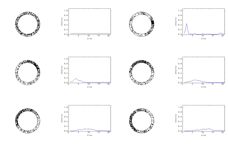
Anyway, here is an animation of dots being instantly debited from one account (box) and credited to another; I know because I wrote the Mathematica code that does it (feel free to email me via the box on the sidebar for a copy):


It's from this post. There is strict accounting (the number of dots is constant, and one dot taken from one box is exactly matched by a dot added to another). Then Steve asked the question that you'd hope to get if you were teaching this stuff as a class:
Which raises the interesting (for me...) Q: when I send you money, how far does it "move"?

This is an interesting question and in the animation above there is an explicit answer: it moves one box in one time step. In real life, if you gave several people a large amount of money, you could measure how fast it moves from one node in the network to another. One bought dinner here; another bought a record there. The restaurant and music store paid their employees the next Thursday, but the wait staff took home their tips that night and one picked up some groceries. It possibly changed forms during this journey from cash from an ATM or a deposit at one. This data would be an input to a bottoms-up measurement of money velocity.

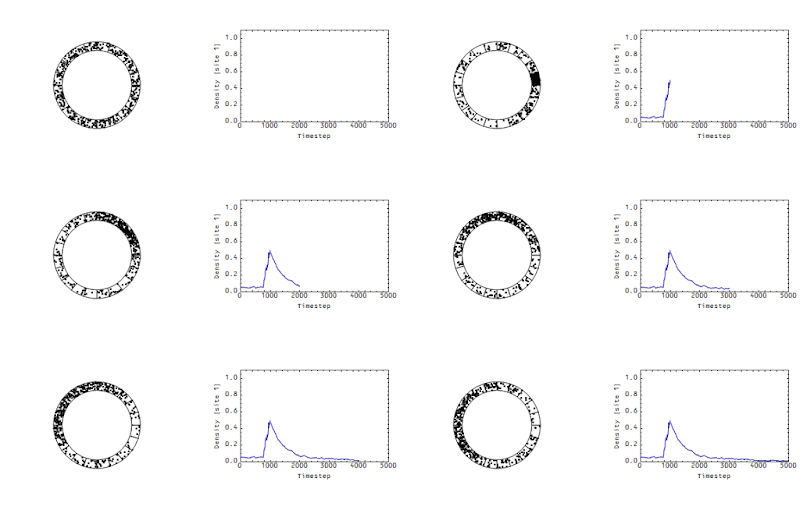
These measurements determine the flow rate of money in an economy analogous to the flow rate of the wave in the animation above. There's another picture from that same post -- it shows the density at a single site:


Note that there's a "decay constant" (of about 500 time steps) -- this decay constant is directly related to the speed of the flow in the first animation. The faster that wave moves in the first animation, the faster the density would decay in the second animation.

I hesitate to bring it up again, but this is exactly what I was talking about when I criticized stock-flow consistent models (Steve also brought up "accounting" approaches).

Even though the accounting is exact in the model above, I could make the wave travel faster or slower (and therefore the decay happen faster or slower) by changing the size of the debits and credits or changing the number of transactions per time step. The velocity of the wave is a free parameter not established by pure accounting. In the linked post, I called that free parameter Γ and was promptly attacked by the stock-flow consistent community for heresy.

So where does this parameter come from? Where does velocity come from? Where does my freedom come from when Nick Rowe says:
But velocity is not just an accounting relationship between flows and stocks. I can choose the velocity of circulation of the money I hold.
Let's consider a set of accounts on a network: I buy something from you, you buy something from someone else, etc. all in a chain (time steps t are vertical, and accounts a are horizontal):


Now, what happens if I do this:


I made the accounts farther apart and the time steps closer together. In terms of accounting? I did nothing. It's just a graphic design choice. That's because these accounting boxes have nothing to do with each other in time and space. However, I've implicitly related them to each other because the boxes "next to" each other are in a sense closer to each other. There is some kind of "connection" between boxes (two are shown in blue):


How do I measure distance diagonally? How is one time step related to one account step? Well, much like how I could make any graphic design choice, I can choose any relationship between a time step Î”t and an accounting step Î”a (I could even make Î”a = Î”a(t) change as a function of time -- an expanding accounting universe). There's a free parameter that comes out of this two-dimensional space time (for flat space). In physics, it's called the speed of light (c). The space steps Î”x are related to time steps Î”t such that distance Î”s is measured with some function

Δs² = f(Δx, c Î”t) = c² Î”t² - Î”

... at least for the those of us on the West Coast.

This is what was so frustrating about the stock-flow argument. The metric was assumed to be analogous to


Δs² = f(Δx, c Î”t) = Î”t² + Î”


as if it was a fundamental accounting error to assume otherwise. Frequently physicists do assume h = c = 1. But then we measure everything in terms of energy or distance. One Fermi is not just a distance but also a time and both are the same as 1/197 MeV (inverse energy) which is also about 1/400 electron masses. That's only because the theory of relativity exists relating energy, matter, space, and time. You could do this in stock flow models -- assuming a new fundamental constant Γ = 1 dollar/quarter -- but then you'd have to measure time in terms of money. A year is not 4 quarters, but rather 4 dollars-1.


Stock flow consistent analysis is not the special relativity of economics and there is no such fundamental constant as Î“. The accounting "metric" changes over time (those time steps can seem pretty fast when there's a recession happening).

Thursday, June 16, 2016

New CPI data, and an IE model gets rejected


There is new CPI data out today, so I've updated the lag model. It looks like it's not doing too well. There's the spike in January/February, which might be transient. It's within 3 sigma (0.03%, or one month in 30 years), but it occurs in both PCE and CPI data which makes it more like 4.5 sigma (one month in 12,000 years -- since the last ice age). That's troubling, but another problem is the IE lag model is consistently under-estimating the last 8 measurements of CPI inflation (there's a bias), which is a 0.4% probability event (about 3 sigma) on its own.

I could try to console myself with the fact that the measurement of CPI inflation changed slightly in January 2016 (they started using an arithmetic mean for prescription drug prices, but that's a small component of CPI). However that doesn't fix the consistent bias. I'll still follow this model however -- the data does show periods of persistent over- and under- shooting.

Note that this is just the lagged-GDP model of CPI inflation (that I'd hoped might squeeze a few basis points more accuracy out of the data), not the PCE inflation model that is in a head-to-head competition with NY Fed DSGE model (see here for the list of predictions).

Wednesday, June 15, 2016

Macroeconomists are weird about theory

Employment rate e = 1, e ≈ 1 - u* (natural rate), and data. The "pool player" isn't that far off.

Noah Smith has a problem with Milton Friedman's "pool player analogy", and his post is generally very good so check it out. However I think it is also a good illustration of how weird economists are with theoretical models -- at least to this physicist.

As an aside, biologist David Sloan Wilson cites Noah approvingly, but possibly does not remember that he (Wilson) said that Friedman's "as if" arguments are evolutionary arguments (that I discussed before, which would also be a good post to look at before or after you read this one).

Anyway, let me paraphrase the pool player analogy:
Pool players operate as if they are optimizing physics equations

Economic agents operate as if they are rational utility optimizers
Noah's objection is that either a) you optimize exactly therefore you don't need to know the physics equations, just the locations of the pockets, or b) you don't optimize and therefore there are a lot of things that go into why you'd miss from psychology to nonlinear dynamics. As he says: "Using physics equations to explain pool is either too much work, or not enough."

This is a false dichotomy, and it results from the general lack of scope conditions in economics. Noah says this is an important topic to think about:
I have not seen economists spend much time thinking about domains of applicability (what physicists usually call 'scope conditions'). But it's an important topic to think about.
I'll say!

[Actually from a Google search, "scope condition" seems like a sociology term. I never used it as a physicist -- rather it was a domain of validity or scale of the theory.]

Mathematically, Noah is saying (if p is the probability of getting a ball in the pocket) either

p = 1

or

p = f(x, y, z, ...)

where f is some function of physics, psychology, biology, etc. This is not what Milton Friedman is saying at all, and isn't how you'd approach this mathematically unless you look at math the weird way many economists do -- as immutable logic rather than as a tool.

Milton Friedman is saying (just keeping one variable for simplicity):

p ≈ 1 + o(x²)

And with pool players in a tournament, that is a better starting point than p ≈ 0. I put o(x²) (here is Wikipedia on order of approximation) because Friedman is saying it is an optimum, so it likely doesn't have any first order corrections. This latter piece may or may not be true, so a more agnostic view would be:

p ≈ 1 + o(x)

So what about the scope conditions? Let's take Noah's example of random inhomogeneities on the balls, the table and in the air. [Update: I want to emphasize that it is the "as if" theory that gives you your hints about how to proceed here. The pool player is operating "as if" he or she is optimizing physics equations, therefore the scales and scope will come from a physics model. This of course can be wrong -- which you should learn when the theory doesn't work. For example, DSGE models can be considered an "as if" theory organizing the effects, but have turned out wrong in the aftermath of the Great Recession.] These have to be measured relative to some size scale S₀ so that we can say:

p ≈ 1 + o(s/S₀)

Now is S₀ big? Maybe. Maybe S₀ represents the table size; in that case the linear term is important for long shots. Maybe S₀ represents the ball size; in that case the linear term is important for shots longer than the ball's diameter. Maybe S₀ is the size of a grain of sand; in that case you might have a highly nonlinear system.

That's what theory is all about! It's all about finding the relevant scales and working with them in formal way. Other uses of mathematical theory are weird.

The second half of Noah's post then asks the question: what if

p ≈ 1

is the wrong starting point -- a "broken piece" of the model? Can a collection of broken pieces result in good model? For example, you could imagine the "bad player approximation"

p ≈ 0

In physics, we'd call p ≈ 1 or p ≈ 0 different "ansätze" (in reality, physicists would take p ≈ c and fit c to data). In economics, these are different "equilibria" (see David Andolfatto on DSGE models; this correspondence is something I noted on Twitter).

The crux of the issue is: do the broken pieces matter? If I think

p ≈ 1 + o(s/S₀)

but you think my model is broken (or contradicts the data), the model could still be fine if s << S₀. Lots of different models ...

p = f(a) ≈ 1 + o(a/A₀)
p = f(b) ≈ 1 + o(b/B₀)
p = f(c) ≈ 1 + o(c/C₀)

... could all lead to that same leading order p ≈ 1. For example, that leading order piece could be universal for a wide variety of dynamical systems (this is quite literally what happens near some phase transitions in statistical mechanics).

What is interesting in this case is that the details of the system don't matter at all. If this were true in economics (we don't know), it might not matter what your Euler equation is in your DSGE model. Who cares if it violates the data -- it might not matter to the conclusions. Of course, in that example, it does matter: the Euler equation drives most of the macro results of DSGE models, but is also rejected by data.

There are many other ways those extra terms might not be important -- another example happens in thermodynamics. It doesn't matter what an atom is -- whether it is a hard sphere,a quantum cloud of electrons surrounding a nucleus, or blueberries -- to figure out the ideal gas law. The relevant scales are the relative size of the mean free path λ ~ (V/N)^(1/3) and the size of the "thing" you are aggregating (for atoms, this is the thermal wavelength, for blueberries is is about 1 cm) and the total number of "things" (N >> 1). (Although blueberries have inelastic collisions with the container, so they'd lose energy over time.)

The other great part about using scope conditions is that you can tell when you are wrong! If the details of the model do matter, then starting from the wrong "equilibrium" will result in "corrections" that have unnatural coefficients (like really big numbers c >> 1 or really small numbers c << 1) or get worse and worse at higher and higher order -- the (s/S₀)² will be more important than the s/S₀ term. This is why comparison to data is important.

But the really big idea here is that you have to start somewhere. I think David Andolfatto puts it well in his DSGE post:
We are all scientists trying to understand the world around us. We use our eyes, ears and other senses to collect data, both qualitative and quantitative. We need some way to interpret/explain this data and, for this purpose, we construct theories ... . Mostly, these theories exist in our brains as informal "half-baked" constructs. ... Often it seems we are not even aware of the implicit assumptions that are necessary to render our views valid. Ideally, we may possess a degree of higher-order awareness--e.g., as when we're aware that we may not be aware of all the assumptions we are making. It's a tricky business. Things are not always a simple as they seem. And to help organize our thinking, it is often useful to construct mathematical representations of our theories--not as a substitute, but as a complement to the other tools in our tool kit (like basic intuition). This is a useful exercise if for no other reason than it forces us to make our assumptions explicit, at least, for a particular thought experiment. We want to make the theory transparent (at least, for those who speak the trade language) and therefore easy to criticize.
Andolfatto is making the case that DSGE is a good starting point.

But this is another place where economists seem weird about theoretical models to this physicist. Usually, that good starting point has something to do with empirical reality. The pool player analogy would start with p ≈ 1 if good players are observed to make most of their shots.

Economists seem to start with not just p ≈ 1 but assert p = 1 independent of the data. There is no scope; they just armchair-theorize that good pool players make all of the shots they take -- turning model-making into a kind of recreational logic.

[Aside: this is in fact false. Real pool players might actually consider a shot they estimate they might have a 50-50 chance of making if they think it might increase their chance of a win in the long run. But still, p ≈ 1 is probably a better leading order approximation than p ≈ 0.]

Sometimes it is said that asserting p = 1 is a good way to be logically consistent, clarify your thinking, or make it easier to argue with you. Andolfatto says so in his post. But then p = 1 can't possibly matter from a theoretical point of view. It's either a) wrong, so you're engaged on a flight of mathematical fancy, b) approximate, so you're already admitting you're wrong at some level and we're just arguing about how wrong (an empirical question), or c) doesn't matter (like in the case of universality above).

In physics we know Newton's laws are incomplete (lack scope) for handling strong gravitational fields, very small things, or speeds near the speed of light. We'd never say that's fine -- let's try and understand micro black holes with F = ma! The problem is compounded because in economics (in macro at least) there aren't many starting points besides supply and demand, expectations, the quantity theory of money, or utility maximization. In physics, there were attempts to use classical non-relativistic physics to understand quantum phenomena and relativity when it was the only thing around. If all I have is a hammer, I'm going to try to use the hammer. We discovered that regular old physics doesn't work when action is ~ h (Planck's constant) or velocity ~ c (speed of light) -- that is to say we discovered the scope conditions of the theory!

What should be done in economics is use e.g. DSGE models to figure out the scope conditions of macroeconomics. DSGE models seemed to work fine (i.e. weren't completely rejected by data) during the Great Moderation. The Great Recession proved many models' undoing. Maybe DSGE models only apply near a macroeconomic steady state?

In general, maybe rational agents only apply near a macroeconomic steady state (i.e. not near a major recession)?

This is what David Glasner calls macrofoundations of micro (the micro economic agents require a macroeconomic equilibrium to be a good description). Instead of repeating myself, just have a look at this post if you're interested.

Overall, we should head into theory with three principles
  1. Models are approximate (every theory is an effective theory)
  2. Understand the scope (the scale of the approximation)
  3. Compare to the data
Do those three things and you'll be fine!

The weird way economists do theory inverts all of these:
  1. Models are logic
  2. Ignore the scope
  3. Data rejects too many good models
If you do the latter, you end up with methodological crisis (you can't fix bad models) and models that have nothing to do with the data -- exactly what seems to have happened in macroeconomics.

...

PS Pfleiderer's chameleon models are ones where they assume p = 1, and try to draw policy conclusions about the real world. When those policy conclusions are accepted, the p = 1 is ignored. If someone questions the model, the p = 1 is described as obviously unrealistic.

PPS Everything I've said above kind of ignores topological effects and other non-perturbative things that can happen in theories in physics. There are probably no topological effects in economics and the picture at the top of this post (from here) doesn't look non-perturbative to me.

Monday, June 13, 2016

The urban environment as information equilibrium


Cameron Murray wrote a post a couple weeks ago that made me think about applying information equilibrium to urban economics. Cameron tells us "[t]he workhorse model of urban economics is the Alonso-Muth-Mills (AMM) model of the mono-centric city" and then goes on to look at some of its faults. Here's his picture:


Let's tackle this with the information equilibrium framework.

Let's set up the information equilibrium system (market) $h : R \rightleftarrows S$ where $h$ is building height (proxy for density), $R$ is distance (range) from the center and $S$ is the supply of housing (housing units). And let's assume $R$ varies slowly compared to $S$ -- i.e. transportation improvements and new modes (that fundamentally change the city's relationship with distance) happen slowly compared to adding housing supply. This puts us in the partial equilibrium regime with $R$ as a "constant information source" (see the paper). Height $h$ is the detector of information flowing from the distance from the center to the housing supply; in economics, we think of this as a "price".

The "market" above is shorthand for the information equilibrium condition (with information transfer index $k$)

$$
h \equiv \frac{dR}{dS} = k \; \frac{R}{S}
$$

which we can solve for slow changes in $R$ relative to $S$ (and then plug into the "price" $h$) to obtain (with free parameters $R_{0}$ and $S_{ref}$ are model parameters):

$$
h = \frac{k R_{0}}{S_{ref}} \exp \left( -\frac{\Delta R}{k R_{0}}\right)
$$

Here's a plot of this function:


You could of course substitute housing price $p$ or density $\rho$ for $h$ (or more rigorously, set up information equilibrium relationships $p \rightleftarrows h$ or $\rho \rightleftarrows h$ so that e.g. $p \sim h^{\alpha}$ so that $p \sim \exp \; -\alpha \Delta R$).

Now markets are not necessarily ideal and therefore information equilibrium does not hold exactly. In fact, it fails in a specific way. The observed height $h^{*} \leq h$ (because the housing supply $S$ can only at best receive all of the information from $R$, i.e. $I(R) \geq I(S)$, a condition called non-ideal information transfer), so what we'd see in practice is something like this:


Here's a logarithmic scale graph:


This is not too different from what is observed (assuming price is in information equilibrium with building height $p \rightleftarrows h$) from here [pdf]:


In short, information equilibrium provides a pretty good first order take as an urban economic model. You can see that height restrictions and other zoning ordinances or preserved green space end up impacting the observed height negatively -- i.e. non-ideal information transfer.

Saturday, June 11, 2016

Unemployment equilibrium?

Earlier today, Roger Farmer tweeted a post of his from a couple years ago that had a line that struck me as odd. It's just an example of something I've read many, many times in economics from papers to the blogs so I'm not singling out Farmer for this. The line was this:
For example, I have constructed a DSGE model where 25% unemployment is an equilibrium.
There are other papers that refer to an unemployment equilibrium. However, is there any sense in which there is an equilibrium in unemployment? Take a look at the data:


Which level would you choose to be the equilibrium? It looks to me like unemployment has never stayed at any particular level for more than a year or two (within error). That 25% unemployment equilibrium (or 5%, or whatever level you can construct with a DSGE model) does not seem to describe an actual macroeconomy.

There is another type of equilibrium in economics; many economies generally grow, sometimes at a roughly constant rate. That exponential growth path can be considered an equilibrium. Maybe we can consider employment growth (and thus unemployment reduction) as an equilibrium path? This is an idea I'd had awhile ago when I noticed that recoveries had a remarkably regular slope. I've made it a bit more scientific for this post.

Imagine setting up a series of diagonal lines. The regions between those diagonal lines can be considered a bin -- if the unemployment rate falls in that bin, it adds to a histogram. You can visualize it like this (I did this by hand, so it doesn't match perfectly):


The question is: is there a slope of those lines (α) such that the histogram is very spiky (most points fall in a few bins)? Technically, I am minimizing the entropy of the distribution over α. It turns out there is:


The value is α = 0.49 (i.e. a 0.49 percentage point decrease in unemployment per year, or a 0.04 percentage point decline per month). Here are the histogram and the unemployment rate shown with lines at that slope shown:


It matches the best with the 1991 recession and the 2001 recession recoveries. Once we've established this slope, we can add the function f(t) ~ α t to the unemployment rate; it causes the recoveries to become horizontal lines (that in the normal data would be falling at the rate -|α| per year) and the recessions transitions to become more vertical:


I fit a series of step functions to this data (red) leaving out the 1980s (the Volcker recessions, which seem different -- both in the original data and in this view). Now we can transform the data and the red functions back to the original unemployment view:


I wanted to note that pre-1980 recessions seem to have a bit larger initial overshoot relative to the post-1980 Great Moderation recessions.

So ... can we say the unemployment rate decline at 0.49 %/year is the unemployment equilibrium? Possibly -- at least if the unemployment rate is always large enough to handle it. A decline at 0.49 %/y couldn't be held up for more than 10 years at the current unemployment rate.

In any case, this is a definition of an unemployment equilibrium that makes sense to me.

...

Update 18 June 2016

Here's Roger Farmer with his take: unemployment has two "regimes": increasing and decreasing. This is largely similar to what I've said above, except I emphasized the decreasing regime because it tends to hold for longer periods of time.

Friday, June 10, 2016

Sleight of hand with the regulator


Just to make explicit the switch from the ordinary mean for the ensemble average to the geometric mean in the time average in Ole Peters paper on the resolution of the St Petersburg paradox (that I talked about yesterday), compare equations (5.2) and (5.7)

$$
\text{(5.2) }\; \langle r \rangle_{N} = \frac{1}{N} \sum_{i = 1}^{N} r_{i}
$$

$$
\text{(5.7) }\; \bar{r}_{T} = \left( \prod_{i = 1}^{T} r_{i} \right)^{1/T}
$$

The probabilities $p_{i}$ of each $r_{i}$ are inserted (there is a tiny subtlety here, but the result is as if one had just mapped $r_{i} \rightarrow N p_{i} r_{i}$ in one case and $r_{i} \rightarrow  r_{i}^{T p_{i}}$ in the other) as one would for an ordinary mean and a geometric mean (absorbing the $1/N$ and $1/T$, respectively):

$$
\text{(5.2a) }\; \langle r \rangle_{N} =  \sum_{i = 1}^{N} p_{i} r_{i}
$$

$$
\text{(5.7a) }\; \bar{r}_{T} =  \prod_{i = 1}^{T} r_{i}^{p_{i}}
$$

There is a notational difference designating the time average, but we could re-write (5.7a) as

$$
\langle r \rangle_{T} =  \prod_{i = 1}^{T} r_{i}^{p_{i}}
$$

Note that $T$ is a dummy index (it is taken to dimensionless infinity later just like $N$), so WOLOG we can take $T \rightarrow N$ and the previous equation can be rewritten:

$$
\langle r \rangle_{N} = \exp \left( \sum_{i = 1}^{N} p_{i} \log r_{i} \right)
$$

Peters takes the logarithm of both (5.2) and (5.7) and $N \rightarrow \infty$ to obtain the final result

$$
\log \langle r \rangle = \log \sum_{i = 1}^{\infty} p_{i} r_{i}
$$

$$
\log \langle r \rangle =  \sum_{i = 1}^{\infty} p_{i} \log r_{i}
$$

The first sum diverges. The second sum converges because the infinity has been regulated

$$
\log r_{i} = \log (w - c + 2^{i-1}) - \log (w)
$$

The regulator entered at the beginning -- by taking the geometric mean.

Thursday, June 9, 2016

Regulators

Cameron Murray has a nice post about ergodicity and a resolution of the St. Petersburg paradox by Ole Peters. I proffered my solution (tongue firmly in cheek) a year ago that I'll repeat again here because it's fun and illustrative. I have some problems with what Peters does that I'll go into below (short version: he's not really demonstrating non-ergodicity, but a kind of false equivalence).

The way the St. Petersburg paradox is usually posed is as a game with an infinite expected payout. You flip a coin and the pot doubles each time heads comes up. As soon as tails comes up, you get what's in the pot. The question is: how much should you put up to play this game? Well, a naive calculation of the expected payout is infinite:

E = (1/2) · 2 + (1/4) · 4 + (1/8) · 8 + ...
E = 1 + 1 + 1 + ...
E = ∞

So you should (if you were rational) put up any amount because the payoff is infinite. Ah, but people don't and there have been several "answers" to this problem over the few hundred years it's been around in this form. I was surprised the real answer wasn't listed in the Wikipedia article (but is available on elsewhere on Wikipedia):

E = (1/2) · 2 + (1/4) · 4 + (1/8) · 8 + ...
E = 1 + 1 + 1 + ...
E = ζ(0)
E = -1/2

This was something of an inside joke for physicists who have studied string theory and the number theory crowd.

The interesting thing (for me at least) is that this problem appears to touch on something that was a serious issue in physics in the 1930s and 40s. It's called regulation; it's not about regulating businesses but rather controlling infinity.

When quantum field theory was being developed, there was a big problem in that many of the calculations turned out to give infinite results for things like the charge of an electron because of the swirl of photons and electron-positron pairs that show up courtesy of quantum mechanics. This is a problem because the charge isn't infinite — it's about 0.0000000000000000002 Coulombs.

The solution was to subtract infinity. This is problematic because there are many types of infinities. Let's look at a couple of integrals. Integrals are a kind of sum (the integral sign is a stylized letter s based on handwriting in the 1600s and 1700s). Ignoring the constant of integration, we have

∫dx/x ~ log x

∫dx ~ x

The first on can be thought of as being related to the sum of

1 + 1/2 + 1/3 + 1/4 + ... + 1/x

and the second

1 + 1 + 1 + ... (x times)

The limit as log(x) goes to infinity is "different" from the limit as x goes to infinity: log(x) - x does not exist as x goes to infinity. However log(x) - log(x+1) does exist (it's zero). The key to solving the problem in physics was to subtract the "same kinds" of infinities. But how do you know if you have the same kinds of infinities? You introduce a "regulator".

A regulator makes the calculation finite in some way. One simple regulator is a cut-off regulator. If you only sum up the first 5 terms of the St. Petersburg paradox, the expected value is 5:

E = 1 + 1 + 1 + 1 + 1 = 5

But note that if you change the cutoff, the answer changes. If it is 3, the expected value is 3:

E = 1 + 1 + 1 = 3

If the cut-off is Λ, the answer is E = Λ. Introducing the cutoff introduces a "scale" that the original "theory" does not have. And since we now have a scale, the answer basically has to be that scale (possibly multiplied by some constant of order 1). I talk more about scales here.

That's a big problem with regulators — they can introduce scales to your theory that you the theorist (not the universe) made up. My choice of cut-off chooses the value of E. One solution is to leave the scale as a free parameter and fit it to data. Ole Peters in his paper mentions that people only put up about €10 to play the game. Therefore we can say Λ = €10, and therefore conclude economics has a scale of €10.

Another regulator used in economics is a discount factor. If we consider this game to be played over a long period of time, we can discount the future payouts by a factor β each time period, so that:

E = 1 + 1 · β + 1 · β² + ... = 1/(1 - β)

In that case, for E = €10, β = 0.9. Note that this gives different results depending on the discount factor (and is even negative for β > 1 [2]). This also introduces a scale. If you look at the discount factors multiplying the nth term, you get a graph that looks like this:


One common way to define the scale is to look at where the function falls to half its value, which means that here the "time scale" T is about 7 (i.e. 7 time periods). Here, time is money so this time scale T is related to the term cutoff Î›.

Introducing a scale isn't necessarily problematic; sometimes you know they exist from other reasons. For example, if the St. Petersburg paradox took one year per turn, a human lifetime might be a reasonable cutoff. In physical problems, we can sometimes cut off things at the size of atoms (materials stop behaving like continuous solids at that scale).

However there is an additional issue with regulators: they can break the symmetries of your system. This was a big issue with regulating the infinities in quantum field theory. Regulators like a cutoff aren't Lorentz invariant (i.e. violate the symmetries of special relativity) or gauge invariant (violating the gauge symmetry of the electromagnetic force). Other regulators have been introduced (e.g. Pauli-Villars, which can be used to keep gauge symmetry for QED but not QCD, and dimensional regulation, which involves saying we live in 4 - ε dimensions which is Lorentz and gauge invariant but can mess up other things).

Going back to my joke above, I used what is called zeta function regularization, which basically makes all the real numbers a little bit complex and figures out values by analytic continuation. This can regulate the infinity without introducing a scale or breaking symmetries. The result however is pretty abstract and hard to interpret.

As Peters writes in his paper, Bernoulli solved the problem by introducing diminishing marginal utility with a utility function U(x) ~ log x, adding in the starting wealth of the player w, accounting for the cost to play/bet c, and subtracting off the utility of the starting wealth. This accomplishes the same goal of introducing the discount factor above. This changes the problem to:

U[E] = (1/2) · (log(w - c + 2) - log(w)) 
                + (1/4) · (log(w - c + 4) - log(w)) 
                + (1/8) · (log(w - c + 8) - log(w)) + ...

[Side note, I turned this expression into an integral and evaluated it and the final result does depend on w for small bets c << w so we can consider w the scale introduced, but the expression is a bit ungainly and not very edifying.]

According to the paper, Peters obtains this expression again by looking at the time average growth rate g such that w(t) = w exp(g t). It actually comes before the time average in the paper, but Peters also looks at an ensemble average expectation and comes up with a divergent result. He declares the process to be non-ergodic (time average and ensemble average give different results).

I have issues with the way Peters does the two sums. For one, the time average is a geometric mean and the ensemble average is an ordinary mean. This geometric mean sneaks in the logarithmic utility function because

(x1 x2 x3 ...)^(1/n) = exp((1/n)*(log x1 + log x2 + log x3 + ...))

which is the exponential of the average of the logs. This effectively introduces the utility function with wealth as a scale to regulate the infinite sum in the time average case. In the ensemble average, no regulator is introduced and so the sum diverges.

I was a bit disappointed that Peters result of non-ergodicity comes from regulating the expected value in one case (by using a geometric mean) but not the other. If he had used a geometric mean for the ensemble average, the results would have been the same — and therefore ergodic. Additionally, both would have diverged if an ordinary mean had been used for the time average.

When I started writing this post, I thought this might be a good example of how a) your answer can depend on your regulator, and b) like in the cases of symmetry in physics described above, your regulator can break properties of your system ... like ergodicity. That is still the main point I'd like to make: the way you regulate your infinities is important and can cause problems (like removing scale invariance [1] or making your result non-ergodic).

...

Update + 2 hours

Here's Terry Tao on zeta function regularization. We should think of that function in terms of a cut-off function Î·(n/Λ) so that (with Î› a cut-off scale as above ... or we could use T)

Σ Î·(n/Λ) = -1/2 + C(η,0) Î› + o(1/Λ)

with C(η,0) = ∫ dx Î·(x).

That leading -1/2 is the regularized value of ζ(0) treated as a complex function.

Update + 3 hours

I think, but am not entirely sure, the correct expected winnings for a bet of size c (cost to play the game) is related to the Hurwitz zeta function and is:

E = ζ(0, c + 1) = 1/2 − (c + 1) = − c − 1/2

This is equal to ζ(0) − c (i.e. the expected payoff minus your bet), so is a bit intuitive (if summing 1 + 1 + 1 + 1 + ... can be considered in any way intuitive).

Update + 7 hours

Went on a tangent on twitter. I used to collect old math and physics books. Since we're talking about the Riemann zeta function, I posted a picture from a book from 1933 showing (for the first time) a 3D visualization of |ζ(s)| (and other complex functions). The authors of the book talked to some mathematicians; they said they'd never visualized them before!

Relief of Riemann zeta function from: Jahnke, Eugen and Emde, Fritz (1933). Tables of functions with formulae and curves.

Update 10 June 2016

Here's a post explicitly showing how Peters managed to sneak the regulator in via the geometric mean.

Update 12 June 2016

Note that you could consider the €10 cutoff to be a probability cutoff of 0.1% — probabilities less than 0.1% are treated as zero.

Also, I was part of an art collective some years ago and had a piece in a gallery show based on the Riemann zeta function:


...

Update 19 January 2020

I think, but am not completely sure, another way to look at it is that Peters' set up of the problem privileges the boundary condition (your starting point), but the divergence/convergence is mostly dependent on the behavior at infinity. (Just jotting down a note to remember in the future.)

...

Footnotes:

[1] To bring this back to the information equilibrium approach, the basic equation has a scale invariance, so introducing a scale to regulate infinities would be problematic.

[2] Added in update. As I've gotten a couple of emails and comments about this, I want to say that this was also an analytic continuation joke.