Saturday, May 31, 2014

Post bump (understanding sticky wages and recessions)


I thought I'd give two neglected (IMHO, quality) posts a bump:
  • Sticky wages, information transfer and piece work (Feb 2014) This is an attempt to understand the origin of sticky wages and questions Roger Farmer's assertion that wages were flexible in the Great Depression.
  • The monetary base as a sand pile (Mar 2014) Some numerical differential equation solving and an analogy where NGDP is the height of a sand pile, the monetary base is the amount of sand and recessions are the inevitable avalanches that result as the height increases. Makes sense of these observations of NGDP.

Friday, May 30, 2014

"Out of sample" predictions with the information transfer model

I understand some of the issues (see here and here) that come up when you try to test a model by fitting it to one subset of the available data and using it to predict values in another subset (that's what I mean by the quotation marks around "out of sample"). However, I thought it might be illuminating to see how much of the data from the period 1960-2014 is needed to accurately model the price level and inflation rate or "predict" generic trends. To that end, I fit the price level model to the data from the periods 1960-1970 (red), 1960-1975, 1960-1980, ... 1960-2005, and 1960-2010 (violet), following a rainbow color scheme (the data is the gray dotted line). In the graph below, I only show the "predicted" values extrapolated from the fits, which start at the vertical lines:


Update 5/30/2014: here are the model equations and parameters.

We can see fairly rapid convergence to the price level after about 25 years of training data (1960-1985), which is shown more clearly in this plot of the fit parameter values:


The interesting piece is that the trend towards a less-steep price level as the monetary base increases (a falling inflation rate, i.e. the effect seen in this graph) is already visible even in the fit to 1960-1970 (red) extrapolated to 1960-2014 -- that is, using the information transfer model, you could have seen the current "lowflation" environment in the US coming in the 1970s (amazingly, when inflation was at its peak).

This finding is more visibly dramatic if you look at the (year-over-year) inflation rate:


The red line is predicting low inflation in the 2000s just from 10 years of data in the 1960s (given the empirical path of the monetary base and NGDP). In fact, the issue that throws off the price level fits from that time and isn't predicted by the extrapolation are the two big spikes in inflation in the 1970s. We saw these before in this post on the 1970s -- attributed (at least in narrative form) to the oil shocks of the time, but could also be related to the "Fisher effect" and expected inflation.

Let me caveat the use of the word "prediction" here. The model uses as input empirical values of the currency component of the monetary base ('M0') and NGDP in the extrapolations. However, the model parameters are fixed in that original 10 years of data. In order to get the current inflation rate, you'd stick the current values of NGDP and M0 into the formula you would have had around since the 1970s (if it had existed at the time). That is, the model predicts a fixed relationship between P, M0 and NGDP and given any two values, fixes (i.e. "predicts") the third.

More on Cobb-Douglas functions and information transfer


Here's a bit more on Cobb-Douglas (CD) functions (previous posts here [1] and here [2]). In Ref [1], I was looking at the Solow growth model which uses a Cobb-Douglas functional form (at least asymptotically):

$$
\text{(1) }Y = c K^{\alpha} L^{\beta}
$$
In Ref [2], I was looking at matching theory which frequently uses a CD ansatz. In my original derivation of a quasi-CD form in the information transfer model in [2], I came up with a function that made a prediction about the exponents in CD forms, i.e.

$$
\text{(2) }Y \sim K^{\kappa - 1} L^{1 - 1/\kappa}
$$

The question is: is this true? If I look at fits to CD production functions or growth models, do they obey Eq (2)? So I went out and tried to do some literature searches and plot the exponents $\alpha$ and $\beta$ (WOLOG, I took the larger exponent to be $\alpha$). There were several papers on the original Cobb-Douglas work from the 1920s (large blue point at $(0.75, 0.25)$ in the graph below for US capital/labor output model), along with several papers on production functions in various industries in different countries. However, the resulting points are by no means exhaustive. In the graph below, $\alpha$ and $\beta$ can fall anywhere in the plot; some models assume constant "returns to scale" such that $\alpha + \beta = 1$, which means the results must fall along the gray line. The information transfer model result (2) above implies that the points must fall along the red line and the red dot at $(0.62, 0.38)$ is the only solution consistent with constant returns to scale. Here is the graph (on the left):


This doesn't look very good. The graph on the right looks a little better, but simply represents plotting $\alpha + \beta$ vs $\alpha$. The most charitable interpretation would be that the information transfer model is predictive of the returns to scale (increasing, constant, diminishing). 

However! During the course of reading a bunch of papers, I came across the "derivation" of the Cobb-Douglas form (it originally comes from the mathematician Cobb who sort of guessed the form based on Euler's theorem, see e.g. here). The derivation posits the basic information transfer model equation I derived in two ways (here and here) as its starting point**. So let's proceed starting from the basic differential equations (we're assuming two markets $p_{1}:Y \rightarrow K$ and $p_{2}:Y \rightarrow L$):

$$
\text{(3a) }\frac{\partial Y}{\partial K} = \frac{1}{\kappa_{1}}\; \frac{Y}{K}
$$

$$
\text{(3b) }\frac{\partial Y}{\partial L} = \frac{1}{\kappa_{2}}\; \frac{Y}{L}
$$

The economics rationale for equations (3a,b) are that the left hand sides are the marginal productivity of capital/labor which are assumed to be proportional to the right hand sides -- the productivity per unit capital/labor. In the information transfer model, the relationship follows from a model of aggregate demand sending information to aggregate supply (capital and labor) where the information transfer is "ideal" i.e. no information loss. The solutions are:

$$
Y(K, L) \sim f(L) K^{1/\kappa_{1}}
$$

$$
Y(K, L) \sim g(K) L^{1/\kappa_{2}}
$$

and therefore we have

$$
\text{(4) } Y(K, L) \sim  K^{1/\kappa_{1}} L^{1/\kappa_{2}}
$$

Equation (4) is the generic Cobb-Douglas form in equation (1). In this case, unlike equation (2), the exponents are free to take on any value. Equation (2) makes more sense when describing matching theory (i.e. a single market $p:V \rightarrow U$), while equation (4) makes more sense when describing multiple interacting markets (or production factors).

** I'd like to point out that assuming a well-known partial differential equation is not very different from assuming its well-known solution -- something I refer to as "ad hoc in the worst way" in an earlier post

Tuesday, May 27, 2014

The Solow growth model and information transfer


Since Piketty has been in the news about economic growth and its relationship with the return on capital, I thought an information-theoretic take on the Solow growth model would be in order.

The Solow growth model basically posits that output is given by a Cobb-Douglas form equation

$$
Y = K^{\alpha} L^{\beta}
$$

I previously applied the information transfer model to Cobb-Douglas form models in matching theory. The same math at that link gives us the information transfer model version of the Solow growth model:

$$
NGDP = K^{\kappa - 1} L^{1 - 1/\kappa} - \lambda_{ref}
$$

The matching theory gives us an interpretation: labor ($L$) is matched with capital ($K$) and creates NGDP. In the information transfer model that becomes: capital transfers information to labor that is detected by NGDP. Let's see how this model does empirically.

I used the real capital stock data from FRED and adjusted it by the CPI (less food, energy) to give the nominal capital stock. Labor is simply the total non-farm employees. The fit parameters for the duration of the data (1957 to 2011, set by the CPI and capital stock data limits, respectively) are $\kappa = 1.51$ and $\lambda_{ref} = 1081$ billion dollars. This means that the exponents don't exactly fit the "constant returns to scale" assumption $\alpha + \beta = 1$. We have $\alpha = 0.51$ and $\beta = 0.34$. The model doesn't do too badly for such a simple model:


It does better on shorter time scales -- here it is fit to 1980-2010:


In the real Solow growth model, $L$ is actually $A \cdot L$ where $A$ represents phlogiston aether technology and knowledge. If we assume that $A$ is reponsible for the deviation from the constant returns to scale between $K$ and $L$, the imputed value of $A$ is given in this graph (normalized to 1 in 1957):

Friday, May 23, 2014

Utility is silly and other observations

Yes, yes, the "marginal revolution" was a huge advance in economics, but when Matt Yglesias referred to total factor productivity as phlogiston economics, I think he missed the real target: utility. I'm going to promote some side comments and random points in a couple of previous posts (here and here) to a post of their own.

If supply and demand is an information transfer process that is related to thermodynamics, then the idea of utility is, well ... silly.

  • The pressure of an ideal gas does not fall because an atom feels the diminishing marginal utility of extra volume. The states of the ideal gas at lower pressure become more likely when the volume is increased. The atoms just blunder into it.
  • The invisible hand of the market is an entropic force. But that entropic force is not encouraging self-regulating behavior of the ideal gas, and it is not channeling atoms' self-interest.
  • If you release a gas into a larger volume (at constant temperature), there will be some fluctuations [1] in the pressure before it settles down to its lower value. However, that doesn't mean there is a "short run" and a "long run" isothermal expansion curve (isotherm).
  • Atoms in an ideal gas don't really have a well defined pressure and volume on their own. Pressure and volume are properties of an ensemble of atoms. Overall, the properties we associate with economic agents are actually only properties of the ensemble system: prices, demand, supply, diminishing marginal utility ... or just utility in general.
  • While some atoms may have a large fraction of the thermal energy of the system, it is largely a function of random chance which atom has which allocation. It doesn't mean high energy atoms are "temperature creators" and the situation would be exactly the same if we re-labeled which atom had which energy allocation. On the other side of the equation, it is hard to alter the velocity distribution from a Maxwell distribution given the macroscopic thermodynamic variables if we leave it up to thermodynamic processes.
[1] The interim state is governed by non-equilibrium thermodynamics and the fluctuation theorem but the information transfer model remains valid under non-equilibrium conditions.

Thursday, May 22, 2014

Limits of the information transfer model

No, this isn't about limitations of the information transfer model. I discussed some of those here. I'm talking about two limiting cases. 

One limit is the high inflation limit; according to this calculation, high inflation means that κ ≈ 1/2 and the information transfer model reduces to the quantity theory of money.

A second limit is the large Monetary Base (currency component) limit. In this calculation, I show that for some value of MB > MB0, we have ∂P/∂MB ≈ 0. This result means changes in the monetary base don't affect the price level P and hence don't strongly affect NGDP. Therefore, in terms of the price level NGDP can be considered approximately constant (aggregate demand is a constant information source) with respect to central bank operations, the IS-LM model is valid for the effects of interest rates and the information transfer model reduces to (Hick's description of) Keynesian economics.

Thus the two big theories of the last century in economics are specific limits of the information transfer model.

Now if I could just attract the attention of the economics Nobel committee ... or really any economist at all.

Causality in the information transfer framework

It doesn't matter where or how the central bank injects liquidity. Image from wikimedia commons.

A quick note on causality because it's come up in a variety of forms recently (I'll use the interest rate model for concreteness):

  1. Can you be sure that the relationship between interest rates and the monetary base will hold if the central bank does X?
  2. Does lowering interest rates cause the monetary base to rise or vice versa?
  3. You say that interest rates can be lowered by the central bank printing currency, but that's not how open market operations work in real life, so the central bank can't lower interest rates by printing currency.
The information transfer model is based on information theory, but also behaves like a kind of generalized thermodynamics. Let's say we have two variables: money m and interest rate r. The idea is that if you change one variable (r1 → r2), then the other variables respond (m1 → m2) not because they are "caused" to do so by "forces", but rather because it is overwhelmingly statistically probable that if r2 becomes true of the macrostate, then the microstates will be in a macrostate described by m2. This is the basic idea behind entropic forces. Money doesn't make its way from bank vaults into a person's hand because of changes in incentives or utility because you changed r and m (well, at least in this model [1]). It makes its way there because the state with the money in a person's hand is far more likely than the state with the money in the vault given the macroeconomic observation of the system in the state (r2, m2). It is not important how the money got there from a macroeconomic perspective.

Imagine bacon cooking in the kitchen. In the diffusion process, the smell fills the house. I do not need to know the actual trajectories of the molecules, or even how much kinteic energy they leave the bacon with. It doesn't matter if the bacon is cooked in the kitchen or in one of the bedrooms -- the smell will fill the whole house.

The thing that is important is that the economy is a large system. In that case, because of the law of large numbers, I can know that the result will converge to the mean and fluctuations around it will be small. Flipping a fair coin 5 times has a lot of uncertainty in the final outcome (4 heads, 1 tail? 2 heads, 3 tails? 5 tails?). Flipping a fair coin 5 million times does not (2.5 million ± 2200 heads).

The law of large numbers means we know that the final state (r2, m2) will be realized with high probability. But it actually doesn't have to be! It could end up as (r2, m1) or (r2, m3). That's why saying r1 → r2 causes m1 → m2 is problematic. The final state m2 is not a foregone conclusion -- there will be some statistical fluctuation around it.

The law of large numbers also lets us know that the reverse causality works. If m1 → m2 then we will have r1 → r2. That's because if the most probable macrostate (r2, m2) is consistent with r2 if we change r, then it is also the most probable macrostate with m2 if we change m. If m1 → m2 but r1 → r3, then (r3, m2) would be the most probable macrostate consistent with m2. This state would have to be more probable than (r2, m2) since it is the most probable macrostate consistent with m2. The only way this is logically consistent with is if r2 = r3. See this link for more on this subject.

So the answers are:
  1. If the model is correct, then yes.
  2. Yes. Both. Or neither. Doesn't matter.
  3. If the model is correct, the particulars of the process do not matter.
[1] This represents a huge break with traditional economics. It also makes traditional economics seem kind of silly if you try to use the language of utility in thermodynamics ... The pressure of an ideal gas falls because an atom has diminishing marginal utility of extra volume. Ha! This break is also interesting because it means that all the properties of supply and demand are emergent. Atoms don't have feelings about pressures and volumes and the idea gas law isn't even true for an individual atom. Bringing this insight back to economics: diminishing marginal utility is not a property of an individual economic agent, but rather an ensemble of agents. Supply and demand is not about incentives, but rather a property of ensembles of people performing market transactions.

Wednesday, May 21, 2014

A starry-eyed aside on methodology

Mark Thoma and Simon Wren-Lewis recently had some discussion of economic methodology, and during the course of writing the past several posts, methodology has been on my mind. I hinted at it here, here, here and here.

Now I'm not here to say "you're doing it wrong" (which would anger Chris House), but I do think economists, econobloggers and econoblogocommenters should have far more skepticism of their conclusions than they seem to have -- especially when it comes to "natural experiments" in macroeconomics (such and such country did X and the result was Y). I also think Stephen Dubner should be legally required to say "This may well be bullshit, but ... " before everything he says.

I am going to illustrate this with an elaborate analogy. Macroeconomics has a difficult time performing reproducible experiments which means that it is primarily an observational science. Just like astronomy -- and that will be the source of the analogy.

The astronomy story

In astronomy, there is an empirical diagram called an HR diagram. It plots stars' luminosity (L) versus their color index (B-V). It makes somewhat of a line (for main sequence stars):


The theoretical framework at the time believed stars converted gravitational energy into thermal radiation as the star shrank in size. However this led to the sun being only millions of years old instead of billions.

Some stars do fluctuate in luminosity and you might think that would be an excellent place to look for a natural experiment. However, the correlation of log L with the color index is -0.86. These variables are highly correlated so "natural experiments" (e.g. watching a star fluctuate in luminosity) are practically useless (you can't be certain of effects you don't know about or haven't controlled for -- you have to assume your model is right). The only resort is to accumulate data from a bunch of different stars that are in different places on the diagram and try to come up with a theory that encompasses the data based on something besides astronomy.

Even though astronomers didn't know where stars got their energy, Eddington managed to explain the basic physics of how the diagram comes about in the 1920s. Thermodynamics says that stellar temperature is related to luminosity, but the required energy is far beyond gravitational or chemical energy. Thermonuclear reactions are required.

The economics story

In macroeconomics, there is an observed empirical relationship between the money supply and the price level. There is a basic theory that says that growth in the price level in the long run is equal to the growth in base money. However this had a problem explaining how Japan's base could grow without causing inflation.

Economic fluctuations do occur, so many economists try to use them as natural experiment. However, the correlation of the price level with the base (or even M2) is 0.95. These variables are highly correlated so "natural experiments" are practically useless (you can't be certain of effects you don't know about or haven't controlled for -- you have to assume your model is right). The only resort is to accumulate data from a bunch of economies and try to come up with a theory that encompasses the data based on something besides macroeconomics. How about this one?


The key to figuring out the HR diagram was applying the right theoretical framework (thermodynamics). But the interpretation of the data is highly framework dependent -- remember the gravitational theory of stellar radiation? Supply and demand, expectations-based theories, DSGE models. These are the frameworks. Looking at macro data and saying fluctuation X is due to cause Y is dependent on those frameworks. Fiscal policy was ineffective in the US because of monetary offset ... in a monetarist AD/AS model. The US is currently stuck in a liquidity trap so monetary policy is ineffective ... in an IS-LM framework. Macro data isn't going to resolve the ambiguities -- it will just add to existing correlations on which those models are based.

As a side note: if money is analogous to the energy source of stars, economics is still in a state of not exactly knowing what that source is, just like Eddington. Not knowing what money is shouldn't be an impasse!


Mildly related update (5/24/2014): There's a big dust up on the political economy side of things with this comment on the data in Piketty's recent book. Overall, I'd like to say that if you look at the blue lines in the later graphs, they're broadly consistent with the red lines (see e.g. Matt Yglesias) so the first several points don't seem to matter that much. But I would like to address one comment made by Giles:
As I have noted, even with heroic assumptions, it is not possible to say anything much about the top 10 per cent share between 1870 and 1960, as the data for the US simply does not exist.

This is where the HR diagram in the post above comes in. Part of the reason we know about the our sun's evolution is that there are hundreds of stars out there in that are similar to our sun at different times in their life cycle. We have several countries in the world out there in economic conditions broadly similar to the US in those earlier times and in most cases, pre-welfare state nations today tend to have Gini coefficients of 0.5-0.6 or higher. That is not an heroic assumption, and Piketty's results are consistent with that back of the envelope estimate.

Tuesday, May 20, 2014

Analysis of Morgan Warstler's proposal

I promised to look into the implications of Morgan Warstler's "GI/CYB" proposal with the information transfer model. You're probably familiar with him and his style if you're a regular econo-blogger or econo-blogo-commenter. And I must apologize to Warstler for a couple of comments of his that fell in the spam folder (that I fished out).

Fitting the information transfer model to the empirical data (see here) comes up with a system where economic shocks are realized as job losses instead of nominal wage cuts -- the classic sticky wages model. Total employment (E) is roughly constrained by the function P ~ NGDP/E where P is the price level.  Another way to say that is that RGDP/E = constant. This is basically Okun's law.

Morgan's proposal should essentially lead to a system where those shocks should be realized as nominal wage cuts instead of increased unemployment, at least in the simplest version of the model. To that end, I used the information transfer model to come up with the size of those nominal wage cuts. I still assumed total employment was constrained by P ~ NGDP/E. Anyway, here are the nominal wage cuts we would have experienced over the course of the post-war period:


It basically follows through in the math that the level of unemployment converts rather directly into the average size of the nominal pay cut. Instead of the Great Recession unemployment, we all would have all taken a 6% pay cut.

Want to make your own ITM S&D diagrams?

I put this diagram in the previous post:


Generic supply and demand diagrams are easy to make in the information transfer model. A generic demand curve is exp(1 - x) and a generic supply curve is exp(x - 1). These equations follow from equations (8a,b) and (9a,b) at this post. These intersect at the equilibrium price p = 1 and quantity supplied/demanded Q = 1, and the units of the x-axis are fractional change. For example, moving from Y = 1 to Y = 1.1 is a 10% increase.

Adding in shifts is basically shifting the argument. A shift Δx (either positive or negative) in the demand curve is exp(1 - (x - Δx)) and it's exp((x - Δx) - 1) for the supply curve.

Monetary offset: what are the assumptions?

In the lively comments on this post, there was some discussion of monetary offset. Mostly for my own benefit I thought I'd go through the monetary offset mechanism and discuss where model assumptions enter. Hopefully, I won't be too off base -- or if I am, it will be corrected in further lively comments.

I made a rather bold claim that monetary offset is at its heart an assumption about the power of monetary policy in a footnote, citing Scott Sumner's paper [pdf]. I'll use that paper as the primary reference for the discussion here. The assumptions will be titled in bold below, with details after -- Vox-style.

AD/AS model

The basic framework for monetary offset Sumner puts forward is the AD/AS model. I'll just link to the wikipedia page for what assumptions that entails. Here is the diagram from Sumner's paper that I'll refer to a couple times below:


The idea is that the central bank is targeting an economic equilibrium (price level or inflation) at A so that a boost in AD to AD' through fiscal stimulus, moving the equilibrium from A to B, implies that the central bank will tighten (or will be expected to tighten), bringing AD' back to AD and the equilibrium back to their target at A.

AS is unaffected

One assumption in the AD/AS model I'd like to pull out is that AS is unaffected by shifts in the AD curve. A different way of putting that is that the equilibrium point A still exists to return to if the fiscal expansion leading to the shift to AD' occurs.

I discuss the possibility of the original equlibrium A not existing in a different context in a post here. The assumption of the AD/AS model is that A does exist after the fiscal stimulus and monetary offset.

The central bank will meet/is meeting/has met its inflation target

This is one that I brought up with Sumner in the comments. The "inflation target" part itself doesn't matter so much -- it could be any number of targets or monetary policy regimes. The argument for monetary offset is that the central bank has a 2% inflation target so that when fiscal policy tries to move from A to B, rasing inflation above 2%, the central bank tightens (or is expected to tighten), bringing inflation back to 2%.

The "liquidity trap" shows how this assumption is important. In a liquidity trap, the central bank can't meet its inflation target, say only 1% inflation vs a 2% inflation target. Liquidity is hoarded -- not chasing goods and driving up the price level. If fiscal policy brings inflation up to 2%, then the central bank shouldn't be expected to offset it -- and if it did that would contradict the 2% inflation target assumption.

The monetarist counter to this (AFAICT) is that the central bank was really targeting 1% inflation, not 2% inflation -- i.e. the original assumption that the central bank was meeting its target.

The Concrete Steppes aren't too vast

I think it was Nick Rowe who came up with the phrase "the people of the Concrete Steppes" to refer to economists, bloggers and commenters who doubted that central banks could manage expectations and give forward guidance to move inflation or output without actually conducting open market operations (or showing what those operations could be) -- taking concrete steps. However, like Sumner's gold mining company analogy, sure the announcement can move markets, but they have to start producing some gold in the long run.

The assumption here is that the required concrete actions by the central bank are not outside the realm of possibility. To put it more economic terms, the commitments by the central bank are credible. I hope this roundabout way of getting to central bank credibility illuminates the model-dependence of the meaning of credible.

In Nick Rowe's argument, the concrete steps required are assumed to be effortless (humans just change their minds). I.e. the concrete steps are always feasible. Expectations based on these not-incredible steps are assumed to carry us from one equilibrium to another.

In general, monetarists assume any inflation target can be credible (maybe not specific cases -- Zimbabwe might not be able to credibly promise 2% inflation, but theoretically there could exist a central bank that has a given inflation target).

This credibility assumption is one that at least partially breaks down in the liquidity trap argument. As Paul Krugman likes to say, the central bank must credibly promise to be irresponsible to produce inflation. Monetarists will to point out that the central bank can still credibly produce deflation in the liquidity trap argument, hence monetary offset mechanism in the diagram at the top of this post still applies. Again, this counterargument is based on the idea that the central bank is meeting its inflation target -- a central bank cannot credibly create disinflation/deflation if it is undershooting its inflation target and fiscal stimulus brings inflation up to its target. (Although maybe the ECB really is actually this irrational? Its inflation target is 2% without fiscal stimulus, which it can't meet, and 1% with?)

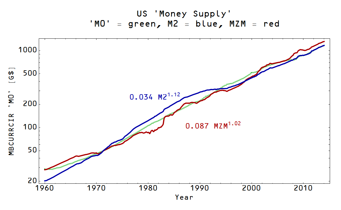
In the information transfer model (ITM), expectations don't matter so much. Regardless of what is expected, the macro variables will generally follow their trends. However the ITM provides an example of the model dependence of credibility. If the monetary base (currency component 'M0') is small relative to NGDP, the assumption of central bank credibility is reasonable. If the base is large relative to NGDP, then some inflation targets may not be credible -- because some inflation rates are impossible in the model. Additionally, the tightening required to offset fiscal policy may be outside the realm of credibility (e.g. taking 10% of currency out of circulation to offset a 3% of NGDP fiscal package, as shown here). This lack of credibility for given inflation rates applies to deflation as well. The idea is that for some economies, ∂P/∂M0 ≈ 0, so both inflation and deflation can require incredibly large increases (decreases) in the monetary base -- if the target price level is even achievable at all.

Small fiscal impacts from monetary policy

One of the things (instruments? tools? this is where the proper technical term should go) central banks use to conduct monetary policy is interest rates. Imagine a budget constrained country with high debt to NGDP; raising interest rates -- considered to be a tightening move by the central bank -- would impact the debt service of that country, impacting the govenment spending package that brought AD to AD' in the diagram at the top of the post. Now the monetary policy required to bring equilibrium B back to equilibrium A is a function of the monetary policy itself! The problem becomes nonlinear and no longer obviously stable to perturbations around the equilibrium A. Additionally, the fiscal impact of debt service can potentially be the same magnitude as the fiscal spending package. In that case, raising interest rates brings you back to equilibrium A without any monetary impact on the price level. This is a bit like finishing building a piece of IKEA furniture and looking back at the box and finding a piece you didn't use.

Before this seems like a just-so story, I'll quote from my response to a comment by Mark Sadowski:
Debt service in Spain jumped fourfold in 2012 after the ECB rate increase, adding 30 G€ in payments, or about 3% of 1 T€ NGDP. Because of the budget constraints, that meant government spending decreased about 3% of NGDP -- accounting for the entire [observed] loss.
I'm not saying this is the definitive answer. This might not be the mechanism that produced the double-dip recession in the EU -- maybe monetary offset is the real reason.

If there are no concrete steps required and the central bank can always meet its targets, the assumption of small fiscal impacts is less of an issue.

More assumptions?

Potential additions in future updates.

Sunday, May 18, 2014

Models matter


This morning I caught Scott Sumner quoting Mark Sadowski:
Now, one can argue that things would have been much worse in the absence of this massive infrastructural spending, but as Kaminska goes on to note, Japan didn’t lose monetary policy traction until much later. In fact the BOJ’s call rate didn’t really hit the zero lower bound until March 1999.
That's the crux of it, isn't it? The monetarist argument is as coherent as the Keynesian argument, so assuming the each side isn't comprised of morons one could argue that things would have been the same or worse (or better!) minus the massive spending by the Japanese government. It's all angels on the head of a pin without a model, though. You need to know that counterfactual. And in order to know the counterfactual, you have to be able to decompose the impact of monetary policy and the impact of fiscal policy.


Let me call up a previous post (and the relevant graph, updated with a red dashed line at a constant interest rate ~ 5%):


The graph shows the impact of an equal percentage increase in NGDP (blue arrows) and MB (red arrows) . For concreteness, let's say a spending package of 3% NGDP [1], or a 3% increase in the currency component of the monetary base. We'll also simplify the discussion by assuming the central bank has an inflation target (this is not an important assumption; the argument still applies if the central bank targets something else like the Fed's dual mandate of stable prices and low unemployment).

This graph is great because it also shows the effect of fiscal and monetary policy on interest rates. Before the 1980s, monetary expansion tended to increase interest rates. After the 1980s, monetary expansion tended to decrease interest rates. This is due to the changing relationship between the income/inflation effect and liquidity effect. Fiscal expansion always increase interest rates (i.e. crowding out).

We can see in the 1960s and 70s, the vectors are not orthogonal. In this world, monetary offset exists. If the government tries to spend more money to cause inflation (blue arrow), the central bank will just make its red arrow slightly smaller (do slightly less expansion) to achieve the inflation target it wants. After the 1990s, the vectors are closer to orthogonal. The central bank has no power to offset fiscal expansion without ludicrous contraction in the base e.g. a ~ 10% decrease in the base might have offset a 3% expansion in 1991 (figure is approximate):


The key takeaway in this post is not the particulars of the model, but rather the capability to show counterfactuals. The information transfer model can decompose the fiscal/monetary vector. The monetarist vs Keynesian/zero lower bound debate is precisely an argument about orthogonality. Monetarists assume the fiscal vector is parallel to the monetary vector; Keynesians assume they are orthogonal at the zero lower bound [2] (Never forget! Modern Keynesians like Paul Krugman assume the vectors are parallel away from the ZLB, just like monetarists). The information transfer model makes no assumptions about being parallel or orthogonal; the relationship comes from the underlying model. The interesting contribution from the information transfer model is to say that both these views are correct ... at different ratios of MB/NGDP.

A side note on the latter part of the quote. Paul Krugman (a proponent of the theory of the zero lower bound) frequently refers to the US and EU being at the "zero lower bound" even though they technically aren't at "zero" (the Fed has an upper bound of 0.25% and the EU was at 1.75% or higher from 2008 until as recently as 2012 and is now at 0.75%). By this usage, Japan was below 1.75% starting in 1995, so the piece at the end about not really being at zero obviously misunderstands the liquidity trap argument. The basic idea behind Keynes was that there is a lower bound to interest rates below which monetary policy will fail to spur people to forego liquidity. Later, this lower bound was considered to be (always) near zero. How do we make sense of Krugman's insistence that the EU at 1.75% was at the ZLB? Because the Taylor rule (or Mankiw's rule) calls for a negative interest rate. It doesn't matter what the actual interest rate is -- actually going to zero would be dandy, but it's because the interest rate favored by a Taylor rule is negative you have a zero lower bound problem. The target interest rate is relevant, but it alone doesn't define a liquidity trap (i.e. the Fed can't set the interest rate at 1% and make the liquidity trap vanish magically).

In the information transfer model, the liquidity trap interest rate depends on the size of the economy and the monetary base. The zero lower bound is only approximately equal to the liquidity trap rate (ZLB ≈ LT).

[1] Note that NGDP = C + I + G + (X − M), so a boost in G to first order increases NGDP. The crowding out effect of government spending is included in the model.

[2] It really is an assumption in the case of monetarists. Don't believe me? Check out Scott Sumner's paper on monetary offset [pdf]. In the first figure it just assumes that it is always possible for AD increase = AD decrease. It assumes the central bank can always hit their targets. For Keynesians, the monetarist position is the assumption. The liquidity trap (orthogonal monetary and fiscal vectors) is derived from something like the IS-LM model at zero interest rate.

Wednesday, May 14, 2014

Switzerland and Sweden

I ran the models for Switzerland and Sweden, the latter because of a comment by Tom Brown here. Neither seem like particularly remarkable cases, and the results fall in line with the results from other countries:


Here is are the model fits for Sweden:


Two major issues. One, the monetary data from Sweden includes an expansion of reserves in the early 1990s that messes with the price level plot. It is supposed to be 'M0' currency in circulation through out, but in the early 1990s the reserves are included (best to ignore the big bump in the early 1990s). Two, Sweden seems to have suffered from interest rate importing (by holding large amounts of foreign currencies) similar to the case in Australia (from the US and UK) in the 1980s, making the monetary base a bad fit to short term interest rates.

To answer Tom's question: negative IOR doesn't appear to impact the data much. It may have prevented deflation (from Sweden's reduction in outstanding currency). Anyway, this should be considered and update to this result (which incorrectly used the full monetary base instead of just the currency component).

Here are the model fits for Switzerland:


One problem is that currency component information is available only through 2006 (from the Swiss central bank), while monetary base data from FRED goes until today. Switzerland also appears to suffer from interest rate importation in the 1980s.

Saturday, May 10, 2014

Do monetary aggregates measure money demand?

I don't know. How's that for a beginning? If we take the currency in circulation (MBCURRCIR at FRED aka 'M0') to be the supply and either M = M2 or MZM to be the demand, we have the solution to the differential equation M = a M0^(1/κ) (first plot, money demand in terms of supply) or it's inverse M0 = b M^κ (second plot, money supply in terms of demand) ... these result in decent, but not amazing fits:


One pedagogical point: in this case the units on each side are the same information-wise (dollars), hence κ doesn't vary when demand is dollars like it does when demand is "dollars of goods and services" (NGDP). Also note that κ ~ 1 in both cases implying that the "price" of money P ~ M0^(1/κ-1) is roughly constant. Another way, the "exchange rate" between demanded money and supplied money is constant.

Friday, May 9, 2014

Adventures in circular reasoning

"[Market monetarists] have a coherent model that incorporates rational expectations and efficient markets."
... Scott Sumner

Efficient markets require rational expectations which is the assumption that expectations are coherent with the model. He goes on to add "We have a model that can explain market responses ..." ... wait, I thought the EMH means that you can't know what the market will do?

Now I actually have learned a lot over the years from Sumner and agree with a lot of stuff that's on his blog. Actually the biggest difference between the information transfer model (ITM) and what seem to be Sumner's views is that many of the things Sumner thinks can happen at any time, the ITM says happens either when the base is low relative to NGDP or high relative to NGDP. Actually that's true of me and about any economist. High interest rates are a sign money's been loose? Yes, but only when the base is small relative to NGDP. Liquidity traps? Yes, but only when the base is large relative to NGDP. Any time there are arguments that derive from the 1970s, they seem to follow in the ITM when the base is small compared to NGDP. Anytime there are arguments that derive from the Depression or Japan since the 1990s, they seem to follow from from the ITM when the base is large compared to NGDP.

In any case, the ITM is a coherent model that incorporates maximally uninformative markets and makes no restriction on expectations.  The ITM distinguishes between the monetary base and currency and understands the temporal aspects of each. The ITM gives an explicit function for the price level and the rate of inflation, unlike Market Monetarists or New Keynesians. It explains the liquidity trap and diminishing effect of monetary expansion. It explains Abenomics. In fact, it gives a coherent view of the history of economic thought and economic performance in the US from before the Great Depression to the present. [1]

What it doesn't have is support [2] from anyone with an economics degree :)

[1] If you read Sumner's linked post, it'll explain the joke.
[2] Noah Smith favoriting my tweets doesn't count.

Thursday, May 8, 2014

Blowing the anti-neo-Fisherite model out of the water

Scott Sumner, to put it lightly, doesn't agree with Noah Smith. And neither does Nick Rowe. The claim is that Canada's inflation target has worked out just fine blows the neo-Fisherite model out of the water. But let's look at where Canada is on my favorite graph of the price level vs the currency component of the monetary base:


Canada is where the US is in the mid-1990s -- still on the highly sloped part of the curve where monetary policy is effective (also note that Sumner quotes Milton Friedman from 1998). The neo-Fisherite piece of the curve is on the right hand side -- where the US was during the depression, where Japan is now and where the US and EU are moving.

Canada shouldn't have a problem hitting its inflation targets yet. Let's check back in 20 years.

Sumner then moves on to say the Fisher effect in interest rates is confusing neo-Fisherites. However, this also doesn't demonstrate anything -- the direction of interest rate changes is well described by the information transfer model (in the diagram below). The Fisher effect only strongly impacted long term interest rates during the 1970s and 1980s. Here's the model diagram (note that the price level vs the monetary base curve is effectively the curve at the top of this post):


Wednesday, May 7, 2014

Equilibrium in a two-good market


Nick Rowe put up a reference post about capital and interest. I thought I'd follow along with the information transfer model. Rowe initially sets up two markets: apples and bananas. If you'd like to start from the beginning with this, here's my original post on information theory in a two good market.

If we solve the equations (8a,b) and (9a,b) in this post for the price in terms of a change in quantity supplied $\Delta Q^{s}$ or demanded $\Delta Q^{d}$, we have

$$
P = p_{0} e^{\Delta Q^{s}/c_{s}} = p_{0} e^{- \Delta Q^{d}/c_{d}}
$$

These equations define supply and demand curves. We'll assume the markets for apples and bananas are independent in the sense that the supply and demand curves for one market don't depend explicitly on the other. This means that if we plot the supply and demand curves for e.g. bananas in the 3D space $(\Delta A^{(s,d)}, \Delta B^{(s,d)}, P)$, they are constant surfaces in the $\Delta A$ (apples) direction, and every slice at constant $\Delta A$ is the same supply and demand curves for bananas. For visual people, pictures are best (bananas on left, apples on right):


The same goes for the apples, but it's constant along the $\Delta B$ direction (on right, above). If I add the supply surfaces prices (times the quantity supplied) for both goods, I get the Production Possibilities (PPS) surface (in relative terms)

$$
PPS = a_{0} \Delta A^{s}  e^{\Delta A^{s}/a_{s}} + b_{0} \Delta B^{s} e^{\Delta B^{s}/b_{s}}
$$

If I do the same for the demands, I get the Indifference Surface (IS):

$$
IS = a_{0} \Delta A^{d}  e^{-\Delta A^{d}/a_{d}} + b_{0} \Delta B^{d}  e^{-\Delta B^{d}/b_{d}}
$$

I plot the PPS in orange and the IS in blue here:


These two surfaces are tangent at the black dot. The locations where $PPS = 0$ represent the production possibilities frontier (PPF), dotted orange curve. This is the line where the total cost to supply the given amount of apples and bananas at particular location on the curve is the same as the cost to supply the amount in equilibrium (i.e. at $\Delta A = \Delta B = 0$ recall we are looking at $\Delta Q^{s}$, not the absolute level $Q^{s}$). Likewise, $IS = 0$ represents the indifference curve (IC). One way to think about these lines is that the represent lines of constant aggregate supply (PPF) and constant aggregate demand (IC) with a changing mix of apples and bananas produced/consumed. In fact, the vertical axis is basically aggregate demand (supply) relative to equilibrium.  By "aggregate" here, we mean just apples and bananas in this two-good economy.

The last piece required to reproduce Rowe's graph is the "budget constraint". This is basically the equation:

$$
a_{0} \Delta A + b_{0} \Delta B = 0
$$

It's the amount you can change quantity of apples or bananas without spending more or less money (note that $a_{0}$ is the equilibrium price of apples). Here are the two curves and the budget constraint, plotted on the same (2D) graph (essentially the slice through zero on the z-axis = relative aggregate demand = relative aggregate supply):


That's all for now. I'll get to the rest of Rowe's post later.

PS Here's another view of those tangent surfaces:

Tuesday, May 6, 2014

Good ad hoc vs bad ad hoc


This goes with this post and Tom Brown's comment asking what I meant by bad ad hoc models. Plastic, like expectations in economics, can be molded into many form factors.

Monday, May 5, 2014

The effect of expectations in economics (third addendum)

Here's a point I left off that didn't fit well in the post from yesterday. In the paper [pdf] Mark Sadowski links to, the mechanism for how expectations enter into the model is illustrated (as an extreme case) in their Figure 1. This is ad hoc in the worst way. The model does not actually add any information aside from the original observation that "calling" a recession has an impact -- a classic example of (the original meaning of) begging the question. If I have an empirical effect and I assume a mathematical model that gives me that effect, what have I learned?

This is an example of what I called the useless power of expectations. I should have been more explicit by calling it the useless power of theoretical models of expectations. I can achieve whatever I'd like by assuming some piece of a model that accomplishes that effect.

For another example, Scott Sumner put forward a verbal model of expectations. Let gold sell at a price p. Sumner first asked what happens if a mining company discovers a huge amount of gold and brings it to market. Well, as supply and demand goes, the price of gold falls. He even provides a just-so story mechanism (the "hot potato effect") whereby individuals unload gold because now there is more gold than individuals want to hold in equilibrium. Eventually the price falls over these transactions until everyone wants to hold as much gold as they have at the new price p'.

Sumner then asks what happens if the company just announces the gold discovery. He says gold prices plunge. I'd agree, but I ask: how far? The worst ad hoc theoretical model of expectations would be to say they fall to p'. But if it's not p', what is it? And why does this new p'' differ from p' derived from the "hot potato effect"? It is possible people will use the heuristic of the relative size of discovery versus the amount of gold previously in the market (e.g. a discovery of 10% the size of the gold market should cause the price to fall about 10%, ceteris paribus). Maybe that heuristic will anchor the expected value at p''. Even then, the distribution of prices achieved [1] in the market grinding down to p' via the "hot potato effect" in the first case will in general differ from the distribution of the expected price p''. Since those probability distributions differ, there is information loss in Hayek's information aggregating function of the price mechanism [2] (i.e. the KL divergence of the two distributions).

This is why rational expectations is one of the only ways forward-looking expectations [3] have been incorporated in economics in a tractable way -- it assumes away the inconsistency between not only the prices p'  and p'', ascribing it to random error, but also the distributions. But that means rational expectations is precisely the assumption that the price falls to p' -- the worst ad hoc theoretical model.

[1] In different possible worlds, the price p' is different -- that's the distribution.

[2] In the information transfer model, we'd say that the information loss due to expectations means that p'' is initially lower than p', eventually drifting back towards p' (ceteris paribus).

[3] Backward-looking expectations (like adaptive expectations or the simple martingale of this post) don't present the same issues as forward-looking expectations. Generally, when these are dramatically wrong it's because of an unforeseen shock.

Sunday, May 4, 2014

Back to the abstract

A frame from the probably-never-to-see-the-light-of-day video introduction to information transfer economics. Additionally, this is probably not an accurate depiction of Fielitz and Borchardt. Graphics borrowed from here.
I saw that Fielitz and Borchardt, whose pre-print inspired me to develop the information transfer model of economics, have added a new reference to economics (in bold) in an update (v3):
Information theory provides shortcuts which allow to deal with complex systems. The basic idea one uses for this purpose is the maximum entropy principle developed by Jaynes. However, an extensions of this maximum entropy principle to systems far from thermal equilibrium or even to non-physical systems is problematic because it requires an adequate choice of constraints. In this paper we apply the information theory in an even more abstract way and propose an information transfer model of natural processes which does not require any choice of adequate constraints. It is, therefore, directly applicable to systems far from thermal equilibrium and to non-physical systems/processes (e.g. biological processes and economical processes). We demonstrate the validity and the applicability of the information transfer concept by three well understood physical processes. As an interesting astronomical application we will show that the information transfer concept allows to rationalize and to quantify the K effect.

I wonder if they saw my blog? I have about 1000 pageviews from Germany ...

UPDATE! I forgot this blog's first birthday! I just noticed the date on the first post (linked up at the top) was April 24, 2013. As a little celebration, here are the top three posts since the blog's inception (I'm actually really proud of all three of these):

1. How money transfers information

2. Entropy and microfoundations

3. The link between the monetary base and interest rates

The effect of expectations in economics (second addendum)

Just a little graph for thought: I went and looked at the distributions of the difference between the empirical and theoretical short term (3-month) interest rate curves from this post when separated into positive and negative differences. I'll suggestively put it up next to the KL divergence graph from this post ...


Hmm ...

The effect of expectations in economics (addendum)

I mentioned in the previous post that I would show and updated diagram:
In thinking about this while writing this post, maybe the theoretical price [interest rate] should be fit to the empirical data (as is done here) instead of being fit to an upper bound of the empirical data as is done above [in the post]. This solution would represent the gray "least informative prior" solution running through the data and the blue more accurate expectations would rise above the theoretical curve and the inaccurate expectations would still fall below the theoretical curve. I will update with this version in a follow-up post.
Here is the new graph:


In this presentation, the theoretical model curve (dark gray) follows the peak of the least informative prior (gray histogram). The incorrect expectations (red histogram) match up with negative deviations and the more accurate expectations (blue histogram) match up with the positive deviations.

For completeness, here is the fit to the short term (3-month) interest rate (the graph above falls in the gray box):