More goodness from Nick Rowe

It's a beautiful Saturday here in Seattle, so I'll make this quick (and somewhat out of order). Nick Rowe has new post up where he puts a few ideas very clearly:

Nominal demand can fall, but it can't fall to zero, unless the stock of base money falls to zero too. And central banks can stop it falling to zero, ZLB or not.

This is basically what happens in the information transfer model -- the existence of money means that the economy can't deviate too far from the NGDP-M0 path without some randomly irrationally exuberant people stepping in and cleaning up.

So any Neo-Wicksellian model with a ZLB must have currency in the model implicitly, even if it's not there explicitly.

Something of a side note on this one: I think that ZLB comes from the existence of money -- an asset that pays a 0% nominal interest rate; that's how it enters implicitly. If you think the ZLB is important, you're implicitly assuming currency. (I think that is the traditional economics answer.)

This next one is a long one:

If the central bank permanently raises the nominal interest rate, will this result in higher or lower inflation? If you tell me what permanently raising the nominal interest rate does to the base money supply growth rate, I can answer your question. If it causes the base money growth rate to increase permanently, like in John Cochrane's model, then inflation will increase. If it causes base money growth to decrease, then inflation will decrease. Tell me how the central bank raises interest rates, and what it is doing with base money growth when it does this. 

So why not just change the question? Ask what happens to inflation and nominal interest rates if the central bank permanently increases the money growth rate? Inflation and nominal interest rates will eventually increase too. What happens to inflation and nominal interest rates immediately is a little more complicated. It depends on whether prices and inflation are sticky, and on how quickly expectations adjust and people learn that the increase is permanent.

This is what I tackled in these two posts:

http://informationtransfereconomics.blogspot.com/2014/09/the-path-of-policy-is-strongly.html

http://informationtransfereconomics.blogspot.com/2014/09/the-liquidity-effect-and.html

And yes, the result is complicated, but it doesn't have to do with expectations or the ZLB (I have explicit money in this model, not implicit, so the ZLB is not relevant), but rather the relative size of the monetary base and the size of the economy. There is a way to translate expectations into this measure if you like expectations more.

Assume a (neo-Fisherite) can opener

Nick Rowe tries to explain the paper [pdf] from Schmitt-Grohe and Uribe. I think I have a shorter version: Schmitt-Grohe and Uribe simply assume their result. They invented a new "lack of confidence shock" with different dynamics that leads directly to the result -- 'confidence' is directly proportional to the nominal interest rate so a higher interest rate brings inflation up and a lower interest rate brings inflation down. Basically, if the central bank sets a higher interest rate in a liquidity trap then people think the economy is going to improve, and, voilà, expectations of improvement lead to improvement.

Now I am interested in the neo-Fisherite view where low interest rates lead to lower inflation -- the information transfer model (ITM) gives that result. However the result in the ITM follows from trying to fit data from before the liquidity trap happened -- it doesn't assume different inflation dynamics in a liquidity trap.

In which I agree with John Cochrane (again)

A rising in nominal interest rate leading to a dip in inflation followed by increased inflation.

When John Cochrane says it -- Noah Smith is all twitterpated and Nick Rowe is moony-eyed; when I say it -- Noah deletes the comment from his blog post [no link, naturally] and Nick calls me warped. So it goes.

Anyway, Cochrane put out a working paper the other day that's set the econoblogosphere alight and Tom Brown asked for a response from me. I'll just work from the most recent post from Cochrane. I'm a little surprised at how much I've been agreeing with him lately.

The subject this time? The neo-Fisherite rebellion. I'm not fully a neo-Fisherite, but I'm sympathetic to many of the ideas and mechanisms.

There are two major ideas Cochrane considers:

1. Raising nominal interest rates can result in inflation.

He allows that it might cause a bit of deflation before and then result in inflation. I pretty much showed that, depending on the path of policy, this is what happens in the information transfer model. I discuss it in this post where I tried to reproduce the results as Stephen Williamson:

http://informationtransfereconomics.blogspot.com/2014/09/the-path-of-policy-is-strongly.html

One of the graphs from that post is at the top of this post. Of course, as I mention in the post on Williamson, something gets in the way: the fact that there is no stable result with a permanent increase in interest rates. Guess what Cochrane' second consideration is?

2. If the Fed permanently pegs interest rates, is inflation stable or unstable in the long run?

I mentioned in the link on Williamson above that there is no stable path of the economy with a permanent increase in interest rates in the information transfer model. In this older post, I show that in order to have an economy with some constant interest rate and some constant inflation rate, you must have an economy with an increasing RGDP growth rate:

http://informationtransfereconomics.blogspot.com/2013/12/a-delicate-balance-part-2.html

Cochrane also puts together a list of ideas that have been "demolished" ...

... MV = PY. Sorry, we loved you. But when reserves go from \$50 billion to \$3 trillion and nothing at all happens to inflation -- or at most we're arguing about percentage points -- it has to go out the window.

This is exactly what I've said here two days before:

http://informationtransfereconomics.blogspot.com/2014/11/quantitative-easing-cleanest-experiment.html

There still is an equation of exchange, but the real equation is log P ~ k(Y, M) log M where k is a function.

... Keynesian deflationary spirals. Just as much as monetarists worried about hyperinflation, Keyensians' forecast of a deflationary spiral just didn't happen.

For this one, I'd say read any post on this blog about inflation. The price level is a function of M and NGDP, and doesn't depend (in the long run) on the expectations involved in the spiral. The only way deflation can happen is either though directly affecting M. In Sweden, the central bank decided to take some currency out of circulation -- and got deflation. In Japan there's a different effect; the currency in circulation has expanded so much that the average information content of each Yen is falling, resulting in deflation.

... The Philips curve. Unemployment went to levels not seen since the great depression; the output gap went to 10 percent and ... inflation moved less than one percent.

Unemployment and inflation trends are pretty unrelated, first here:

http://informationtransfereconomics.blogspot.com/2013/10/the-phillips-curve.html

And in a more recent update here:

http://informationtransfereconomics.blogspot.com/2014/10/updated-non-existent-3d-phillips-curve.html

Fiscal stimulus... well, we'll take that up another day.

Given Cochrane's priors, I think he'll say it doesn't have a positive effect (at least). But if he comes with the answer that's right (ha!) rather than the one he likes, let me tell you what that answer should be -- at least according to the information transfer model.

Fiscal policy has an impact when monetary policy doesn't, such as in a liquidity trap (or generally when the monetary base is large relative to the size of the economy). The two "forces" are orthogonal in a liquidity trap and are closer to parallel when the quantity theory of money applies.

http://informationtransfereconomics.blogspot.com/2014/05/models-matter.html

It's pretty amazing that all this comes from some simple considerations stemming from the idea of money transferring information.

Maybe it should be called the ignorance equilibrium model?

In a brief email exchange about the information transfer model with Robin Hanson, one of the more original and insightful thinkers around today (I read his blog regularly, though I expect roughly a 50/50 chance of disagreeing with a given post -- maybe we disagree on the process of developing our priors [1]), is understandably skeptical and asked a very good question. I am paraphrasing (these are my words, not his), but the essence of the question was: economists have been using information theory for 50+ years, so do you really think you have something new?

This post is going to be an open response to that question and hopefully serve as notes for a future conversation. Please add your comments or criticisms!

I can probably sum up the reason I think I have something different (and as I mentioned to Hanson, the difference may be that it is wrong) in a single sentence: traditional economics puts fathomable human minds at the center of the enterprise whereas information transfer economics assumes humans are inscrutable.

Now I was aware of the importance of information in economics -- my second post on this blog mentions information economics in a postscript:

PS -- While it might eventually be related, the work presented here has nothing immediately to do with "information economics" a la Akerlof, Stiglitz, etc. "Information" is being used in the Shannon sense: a price is communicating a signal from the demand to the supply.

I should have said the price is detecting a signal sent from the demand to the supply, but otherwise that postscript stands up pretty well. The Nobel prize-winning authors I cited are the big names in information asymmetry, where either the seller (usually) or the buyer has more information about the quality of the good being sold. Akerlof showed in his The Market for Lemons that information asymmetry typically drives the value of goods down (or may lead to a lack of any sales at all) and I originally thought this had something to do with non-ideal information transfer where the non-ideal price P* ≤ P (the ideal price) that derives from I(S) ≤ I(D) -- the information received by the supply is at best equal to the information transmitted by the demand.

In the information transfer framework, information asymmetry is a form of non-ideal information transfer. However, in that sentence, the word "information" is being used in two distinct ways. In information asymmetry, a large amount of information about the quality of a good selects a more specific economic state (e.g. quality Q, price P) and thus represents a small amount of information (a small number of possible states consistent with the macroscopic parameters) transferred by the market. A market operating where the demand has a complete lack of knowledge about the quality of a good (i.e. a uniform distribution over Q) has the potential to transfer a large amount of information (a large number of possible states consistent with the macroscopic parameters) ... as long as the supply has an equal uniform distribution.

Ideal information transfer in this case is where the expected distribution over Q on the demand side (call it Qd) the distribution over Q on the supply side (Qs) are equal, Qd = Qs. If they differ, there is information loss -- measured by e.g. the Kullback–Leibler divergence D so that D(Qd || Qs) = D(Qd || Qd) = 0 in the ideal case.

The information asymmetry argument is then that Qs is some tight distribution around the actual quality Q0 while Qd is more diffused (and may not even cover Q0). In this case 0 ≤ D(Qd || Qs), and, in this toy model, I(D) ~ I(S) – D(Qd || Qs) so that P* ≤ P. In the information transfer picture, however, the value Q0 is not relevant and Qs could be narrow around Q1 ≠ Q0 and the result would be the same. What matters is the difference between Qs and Qd, not the accuracy of either estimate.

What is interesting is that in the information transfer model the approximation I(D) ~ I(S) on average, meaning Qd and Qs are on average effectively [2] the same, is a really good approximation for macroeconomic variables (here we've changed Q to mean any relevant metric, e.g. expected NGDP).

Information asymmetry is not important in the generic scenario: it is either always present (see footnote [2]) or always absent. It may have relevance to the dynamics of recession (e.g. it may suddenly change) -- I don't know. However, information loss not important to first order.

Hanson pointed me to Robert Aumann [1] and John Harsanyi, Nobel prize-winners for their research in game theory, specifically on repeated games and Bayesian games, respectively.

The information transfer model in no way invalidates the many insights into microeconomics from game theory, and in fact has little to do with game theory. How do I know? Game theory is a representation of economic microfoundations; the information transfer framework makes as few assumptions about microfoundations as possible. We are assuming we don't know any game theory.

The following is a rough sketch, but one way to think about the information transfer model is as an ensemble of games with random payoff matrices [3] (zero-sum and not) with players repeating games, switching between games and possessing some correct and/or potentially incorrect information about the payoff matrix (or its probability distribution). The only "constraint" is that all of the realized payoffs sum up to a macroeconomic observable like NGDP [3].

The information transfer approach assumes maximum ignorance (maximum entropy) about the players, payoff matrices and strategies (let those define the microstates), that each microstate consistent with the macroeconomic observable (e.g. NGDP) is equally probable.

You could imagine that in such a model, a spreading malaise where investors feel they have insight into the payoff matrices such that the optimal strategy is not to play. Other possible correlated equilibria could appear. A correlation in strategies would represent a fall in entropy (less ignorance about the microstates) and a fall in NGDP (a recession).

This illuminates how the information transfer model differs from game theoretic takes -- regardless of whether they use perfect information, complete information or incomplete information. A correlated equilibrium or Nash equilibrium where there is some optimal strategy that maximizes the payoff (imagine tit-for-tat as applied to the prisoner's dilemma) represents selecting a particular microstate (or set of microstates) which represents a massive loss of ignorance (entropy) of the microstates. That equates to a loss of NGDP relative to players having a random strategy.

One of the issues with the word "information" in information theory is that it is sometimes confused with news or facts, but what is being equated on either side of I(D) = I(S) is the ignorance of the microstates. That ignorance is what is being transferred from demand to the supply. I(D) = I(S) then represents an "ignorance equilibrium". In this model, money is about moving ignorance around.

In searching through the internet, the primary association between economics and information theory the way I am using it is though statistical measures. For example, the Theil index uses information in the same way the information transfer model does. But that is a construction of a particular metric and teasing out the dependence of macroeconomic outcomes on inequality may well be outside the scope of informaiton transfer economics.

The biggest reason I think this is different from previous work in economics -- and maybe some of you out there can help me with this since Google will skew its results based on who is searching -- is that when I do a google image search on "information theory" GDP I mostly get back my own graphs. Have a go yourself:

http://www.google.com/search?q=%22information+theory%22+GDP&tbm=isch

And a search through Google scholar turns up nothing related:

http://scholar.google.com/scholar?q=%22information+theory%22+GDP

An additional reason for believing I am approaching economics in an entirely different way is found in this quote from the textbook (from 2008) linked here (I chose this quote because it puts the idea so concisely):

It is important to note that any definition of supply and demand functions should satisfy two conditions. It should reflect the concrete decision-making of producers and consumers, and it should be founded empirically.

I think this sums up the mainstream view. However, according to information transfer economics, the first condition is not just unnecessary -- it is totally wrong. You assume complete ignorance of the concrete decision-making of producers and consumers. The fact that you give this up -- a deeply held belief that human decision-making is important -- makes me think few economists, if any, have tried this approach. It's a bit like asking if physicists have ever considered a theory where energy isn't conserved. You don't really have to know the literature to say that such theories probably fall outside the mainstream -- even if it was empirically accurate.

Yet another reason is that it has been nigh impossible to find models of the price level -- there are a couple out there, but none use information theory.

If anyone else out there knows of some work that closely resembles information transfer economics, let me know!

Footnotes:

[1] Aumann's agreement theorem is quite useful if you find yourself disagreeing with someone you suspect of being a Bayesian.

[2] Note this may mean that I(D) ~ I(S) + C or a I(D) ~ I(S), where C is some unknown information scale or a is some unknown dimensionless parameter a < 1 that is characteristic of economic processes. We don't necessarily know what the absolute value is for I(D). However, we could just redefine I*(D) = I(D) – C or I*(D) = a I(D) and proceed as if we did know.

[3] Random payoff matrices have been treated in the literature; here are two papers I've found [pdf]:

http://people.hss.caltech.edu/~miaryc/PEW/Michael_Chwe_PEWCaltech.pdf

http://www.ssc.wisc.edu/~whs/research/rdp.pdf

Neither are related to information transfer economics.

[4] One could put expected payoffs and expected NGDP here as well.

Quantitative Easing: cleanest experiment ever?

I'm going to take off my information transfer economics hat and put on my scientist lab coat for this post. I'm going to put forward the idea that the quantitative easing (QE) undertaken by the Federal Reserve was in fact the cleanest macroeconomic experiment ever conducted.

We have a variable that changes decisively by orders of magnitude at a specific time -- and where we know to a high degree of accuracy the counterfactual path of that variable. This variable is the central bank reserves. In the following graph we have the full monetary base (which includes reserves, we'll call MB, blue) and the currency component of the monetary base (which doesn't include reserves, M0, red):

The onset of QE 1 (the first round of QE) happens in November 2008; if we were in grade school science class, that's the moment we connected the battery to the light bulb. 

What do we observe?

Here are the graphs of the 10-year treasury rate ('long' rate, RL, red) and the 3-month secondary market rate ('short' rate, RS, blue). Alongside, I've graphed the ratio NGDP/MB (blue) and NGDP/M0 (red) [1]

Before QE, NGDP/MB, NGDP/M0, RL and RS were all highly correlated. Before QE, it was actually impossible to figure out if any of these variables had anything to do with each other, or if it was just spurious correlation. QE starts and RS falls precipitously. We put the battery leads on the terminals and the blue light lit up.

This happens in several countries by the way (just search on interest rates in the search box on this blog). The experiment was reproducible. I do want to note that Nick Rowe comes close to this measure in this post, except he used M2 instead of M0 or MB.

What else do we observe?

Well, economists have noted for a long time that the price level P and the money supply seem to be correlated, especially during periods of high inflation. Let's plot the Pearson's correlation coefficient of MB (blue) and M0 (red) with P (as well as the correlation of MB and M0, green):

Before QE, all of these are fairly highly correlated -- actually MB and M0 are almost perfectly correlated. This really doesn't tell us very much. NGDP is also highly correlated with the price level. So is population, and in fact any exponentially growing variable.

With the onset of QE, the correlation between MB and P drops precipitously (as well as the correlation between M0 and MB). We see that the counterfactual path MB without QE would have been more correlated with P (effectively given by the red line). We attached the battery leads to the terminal and the blue light didn't light up (the red light stayed lit).

This means central bank reserves have nothing to do with the price level or inflation. Now this doesn't prove that M0 does have something to do with inflation, just that central bank reserves have nothing to do with inflation.

Now there are two arguments out there against this. The first is: the inflation data has been faked. Maybe it has, but realize that same data is the basis for believing the original correlation in the first place. The second is: the central bank reserves are expected to vanish. To me, this is a bit like saying the blue light didn't light because the light bulb expects the battery to be taken away. My counter-argument is Japan:

Both MB and M0 become uncorrelated with P (in fact, they become anti-correlated), so not only does Japan expect the reserves to be taken away, but, as time goes on, a greater and greater portion of the currency in circulation? For each Yen that is printed the market thinks the central bank will take not just that Yen out of circulation, but a second one as well? Additionally, MB and M0 never become uncorrelated with each other -- there never was any large (i.e. order of magnitude) changes in MB in Japan until very recently. There is really no evidence from Japan that MB and M0 are any different from each other -- at least in terms of the price level (MB still is directly related to short term interest rates in Japan like in the pictures above).

This remarkably clean experiment has taught us two things:

1. Central bank reserves are directly connected to short term interest rates.
2. Central bank reserves are unrelated to inflation.

Anyone claiming otherwise is making a strongly counterintuitive claim that, given the uniformativeness of macroeconomic data in general, should be considered speculative at best.

[1] In physics, we like make dimensional analysis arguments (asking 'what else could it be?' about various combinations of scales like masses and lengths) -- if the interest rate with dimensions (units) of 1/year is related to the money supply M (with units of dollars) then it will have to coupled with something with the units of dollars/year -- NGDP fits the bill. Nominal wages and government spending also fit the bill -- however, each of these is highly correlated with NGDP.

Expectations (rational or otherwise) and information loss

The market expectation for NGDP (B, orange) and the actual distribution (A, blue).

This is going to be a rough sketch of an argument and a derivation. The one sentence summary is that there is always information loss in an economy, and that information loss is measured by a combination of NGDP and inflation.

Let's say that the market has an expectation of future NGDP measured by some distribution B; let's call the actual [1] distribution of A. Cartoons of these two distributions are shown in the graph at the top of this post. The difference between these two distributions, measured by e.g. the KL divergence, is:

$$
D_{KL} (A || B) = \Delta I
$$

This is the information gained by learning the real distribution A given distribution B, or alternatively, the information lost by assuming B. I previously talked about expectations destroying information -- they lead to information loss -- here (there's also bit on on the KL divergence). This information loss means that the future NGDP will be lower than the "ideal" NGDP since information in the source (aggregate demand) was not captured at the destination (aggregate supply). Another way to put this is that economic growth is lower than it could be if we knew the future as well as it could be known (i.e. knowing A).

Let's define this ideal (zero information loss) NGDP; we'll call it $N^{*}$ -- measured (observed) NGDP will be denoted $N$. Now the information loss should be equal to the difference in the "economic entropy" (see here, here) of these two NGDPs (I'll work in "natural" units where the parameter $c_{0} = 1$):

$$
\Delta I = \log N^{*} ! - \log N !
$$

Information and entropy are essentially the same thing, just with different units. Using Stirling's approximation for large $N$, we can write this as

$$
\Delta I = N^{*} \log N^{*} - N \log N
$$

Dividing through by the monetary aggregate that defines the unit of account $M$, we get:

$$
\frac{\Delta I}{M} = \frac{N^{*}}{M} \log N^{*} - \frac{N}{M} \log N
$$

And using the information transfer differential equation $dN/dM \sim (1/\kappa) N/M$, we can say:

$$
\frac{\Delta I}{M} = \kappa \frac{dN^{*}}{dM} \log N^{*} - \kappa \frac{dN}{dM} \log N
$$

Let's identify the ideal NGDP with the shock-less NGDP that defines inflation (and is the result of numerically integrating that differential equation without shocks) so that we can use $d N^{*}/dM \sim P$ where $P$ is the price level and $N^{*} \sim M^{1/\kappa}$.

$$
\frac{\Delta I}{M} = P \log M - \kappa \frac{dN}{dM} \log N
$$

Divide through by $\log M$

$$
\frac{\Delta I}{M \log M} = P - \kappa \frac{dN}{dM} \frac{\log N}{\log M}
$$

Using the definition of the information transfer index $\kappa$, we finally obtain:

$$
\text{(1) } \frac{\Delta I}{M \log M} = P - \frac{dN}{dM} = \frac{dN^{*}}{dM} - \frac{dN}{dM}
$$

The information loss is proportional to the difference between the growth rates of the ideal NGDP (also known as the price level $P$) and the observed NGDP ($N$) with respect to the monetary aggregate that defines the unit of account ($M$) [2].

Some observations:

• Rational expectations is the assumption that the distributions A and B are equal, that the information loss $\Delta I = 0$ and that $dN/dM = P$. This is empirically false (what we really have is $dN^{*}/dM = P$). While rational expectations may be a good first order approximation (over the short run), the market does not accurately know the distribution from which macro random variables are selected.
• An inflation target or price level target is a target for the first term in equation (1) while a NGDP level or growth rate target is a target for the second term. That is to say, an inflation or price level target is an ideal NGDP target ($N^{*}$) analogous to an NGDP target. Since $\Delta I$ is a priori unknown, setting one target sets the other. Another way to put this same information is that a given inflation target cannot be achieved simultaneously with an NGDP target (such an economy is over-determined).
• It is interesting that if one adds the assumption that $\Delta I$ is stable (e.g. is a stochastic process with unit root), this comes to the same conclusion as Nick Rowe: But we could live in a [self-stabilizing economy] ... if we adopted price level path targeting [i.e. $N^{*}$], or NGDP level path targeting [i.e. $N$]. However, there is no reason to assume $\Delta I$ is stable and the knob that the central bank would turn would be concrete step of adjusting the currency base ("M0"), not setting expectations (i.e. targeting $\Delta I$, which is impossible since the distribution A is fundamentally unknowable -- it requires knowing not only the future, but all possible futures). Nick's post was the inspiration for this one, which I previously mentioned working on here.
• If rational expectations were true (in the model above), NGDP and the price level would not be independent quantities.

Footnotes:

[1] This would be measured using a large number of identical economies and observing the measured NGDP in each economy.

[2] Note this is a growth rate with respect to the monetary aggregate that defines the unit of account unit of account, not time.

The trouble with Nick Rowe's expectations without concrete steps

I've been thinking about how expectations can set macroeconomic variables without "concrete steps", and in particular Nick Rowe's analogy with daylight savings time. I had some brief interaction with Nick in comments on my post here and this can be seen as an counterargument to this post by Nick.

Nick puts forward two analogies where we achieve a real macro outcome but we don't know what the concrete steps are (or there aren't any concrete steps): driving on the right and daylight savings time. In these situations, the government sets an expectation and everyone complies because everyone thinks everyone else will comply (in this model). This motivates the same logic applying for NGDP (and elsewhere inflation) targeting.

The trouble I've been having with this argument comes down to the fact that we as individuals choose which side of the road to drive on or to set our clocks back. Individuals have the power to set their clocks to any time or drive on either side of the road, and individuals enact the concrete steps. Individuals can't turn a wheel or push a button to set inflation or NGDP.

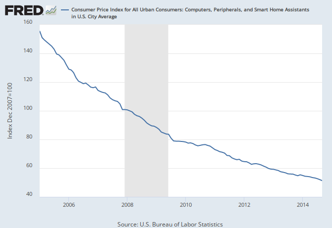
If the central bank set an inflation target and everyone decided to set their prices to rise at 2% per year, then the above analogies seem appropriate. In some cases that could be true: cost of living adjustments, long term contracts, investment decisions, buying a house, etc. However, we as individuals (or even firms) don't make all the choices involved in setting inflation. Some goods actually decrease in price (here is the CPI for computers):

This would be akin to whole segments of the population setting their clocks back when everyone else sets them forward. Additionally, "hedonic" and "quality" adjustments adjustments are made to CPI [1]. The owner of a restaurant can't decide to have prices rise at 3% while having people enjoy the food 1% more. No one can make technology improve based on expectations alone (or can they?).

Unlike daylight savings time or driving on the right, the concrete steps required to enact the inflation or NGDP expectations set by central bank are out of the individual's hands. This is why I reside on the concrete steppes and believe that physical currency ("M0") sets inflation [2], with a changing, but concrete [3], definition of the unit of account.

Footnotes:

[1] PCE inflation measures are highly correlated with CPI and chained CPI, so it would be remarkable if they represented completely independent processes. Without loss of generality, let's stick to CPI inflation.

[2] Empirically, not ideologically -- if it was M1, MB, MZM or any other definition of money, that would be fine by me.

[3] It's very concrete -- the factor is given by the information transfer index and is explicitly κ = (log M0/c) / (log NGDP/c).

Psychohistory? (Qu'est-ce que c'est)

I was reminded of Asimov's psychohistory after reading Igor Carron's post on a new book on signal processing. There were two main axioms (from Wikipedia):

• that the population whose behaviour was modeled should be sufficiently large
• that the population should remain in ignorance of the results of the application of psychohistorical analyses

The theory seems to axiomatically depend on expectations (in economics terms). Knowing the results, in Asimov's galaxy, can influence the outcomes -- hence the rationale for keeping the population in the dark. The information transfer framework mostly depends on the first axiom to produce models, and should produce the same results even if people know about the results of the models -- could it be considered a generalization of psychohistory?

However, Asimov seemed to believe correlations caused things to happen ('mass action'); in the information transfer framework, correlations cause things to fall apart.

Supply and demand for non-ideal information transfer (and other stuff)

Sorry about the lack of posts lately -- I've been busy with with work and on travel. I also discussed actual research money for the model through a (somewhat non-traditional for economics) funding agency and put the idea in front of two professional economists. Understandably, skepticism all around (I have an upcoming post on one of those interactions).

I am also working on a post that started out as a start towards fully incorporating the idea of expectations (as a source of information loss) in response to a piece by Nick Rowe, but Nick has another interesting one that I haven't fully digested yet. Still writing there.

So here's a quick post. Awhile back I did a post on the minimum wage; I used a least informative prior with the non-ideal information transfer to say that the observed price is somewhere in the lower triangle of a supply and demand diagram (see link at the beginning of this sentence for details) -- I don't know where. If we take each position in that lower triangle to be equally probable, then you can show that the centroid appears below the ideal price but at the same quantity supplied/demanded as the ideal equilibrium.

What happens to this point under shifts of the supply and demand curves? Well, it turns out, the non-ideal price follows along a non-ideal supply (or demand) curve that is parallel to the ideal curve. Here's a graph; the purple points represent the starting point and the point after the shift while the dashed purple curve represents the locus of points for different shifts:

Did the Fed cause the Great Recession in the Eurozone?

Scott Sumner's post on Euro-denial among the econ reminded me that I hadn't yet updated the Eurozone trend to account for the strange (and likely not relevant to inflation) impact of 500 € notes. Needless to say, I remain an ECB apologist. It still looks like the big shock of the recession was a result of being above trend:

The secondary shock in 2011 still looks like it came from being above trend as part of a rebound from the lows of 2010. If there is a shock happening now it may well result from external factors like Russia/Ukraine since the data appear fairly close to the trend line.

There was something interesting I saw, however. In this post, I showed that the deviation from the trend in the US in the lead-up to the Great Recession was due to monetary policy by plotting the monetary base on this same graph as M0 (currency). The dotted monetary base line appears to push the M0 curve above the trend and then falls away after the recession (graph reproduced from the linked post):

The monetary base controls the short term interest rates. When the two curves (M0 and MB) approach each other, yield curve inversion becomes more likely, which tends to be a precursor to a recession. The existence of minimum central bank reserves tends to keep the M0 line a constant distance to the left of the MB line. We can see the Fed raising short term interest rates in the mid-2000s and then rapidly lowering them as the Great Recession hits. However, after that, the MB line is so far from the M0 line, it has little to no effect on NGDP (a liquidity trap).

What does this curve look like for the ECB?

It looks like the monetary base has been too large since the inception of the Euro to have any impact on the NGDP-M0 path of the Eurozone economy. It is possible "tight money" (i.e. slow MB growth) pushed the M0 path above the trend in 2010-2011, like a miniature version of the US in 2008. Overall, though, it looks as if short term interest rates (monetary policy) haven't had any traction since 2002. Even with the base expansion, the ECB has mostly been spinning its wheels -- it's been in a liquidity trap this whole time.

Sumner puts the expert witness [3] on the stand:

But the ECB wasn’t even close to the zero bound in 2008.  I get that people don’t like NGDP growth as an indicator of monetary policy, and want “concrete steppes.”  Well the ECB raised rates in 2008. The ECB is standing over the body with a revolver in its hand. ... And then three years later they do it again.  Rates were already above the zero bound in early 2011, and then the ECB raised them again. Twice.  The ECB is now a serial killer.

The liquidity trap has little to do with the zero lower bound (although there is a sense in which they tend to occur together). Interest rates were already too low to move the economy in 2008 and continued to be low through 2011 (the MB curve was well to the right of the M0 curve).

The Eurozone has been like a rudderless ship since the Euro started -- it just so happens that the Great Recession is the only major shock they'd ever had to deal with and the fact that they can't do anything about it makes them look hapless. [1]

But that leaves a question: if the ECB didn't cause the path to rise above the trend (like in the US case), what did? Did the Eurozone import a financial boom from the US? Did the Fed cause the Euro crisis as well as the US recession? Was the ECB framed? [2]

Hmm...

[1] As an aside, I wonder if this explains the strange movements of the Euro monetary base during the Great Recession -- it's like the rudder inputs from a pilot who doesn't know he has lost the rudder, moving side to side, erratically.

[2] I thought about using the title "Has the Eurozone always been in the liquidity trap?" with a nod to The Shining, but Sumner's murder mystery was too much fun.

[3] The economists in denial, per Sumner's accusation.