Vestigial monetarism: Japan edition

A little over a month ago, I wrote a post about how I was laying the last of my "vestigial monetarism" to rest. I didn't explicitly talk about it, but that should also include the monetary model of Japan's consumer price index (last updated here I believe). 

The most recent data (adjusting for the VAT) is actually still consistent with the model:

Unlike a lot of other macro models, this one didn't "die" (H/T Noah Smith) because of Japan but rather because the dynamic equilibrium model of the US data was far more convincing than the equivalent US monetary model (read more about my thinking here).

However, I'll continue to track the dynamic equilibrium model of Japan's CPI (which is (also) doing fine):

Validating employment situation forecasts

The latest employment situation data is out and the latest data is still in line with the forecasts (previous update was here). I've been following the unemployment rate model for over a year now. A lot of people are talking about the increase in labor force participation (there's an especially big spike in "prime age" CLF, but even that spike is consistent with the expected fluctuations in the model. I'll just present the graphs in a gallery (the new data is in black, and the two comparisons are versus various vintages of the FRB SF forecasts and the Fed FOMC forecasts — as always, click for full resolution).

There are two models of the CLF participation rate (one posits an additional shock for reasons explained in a post here):

Also, here's the novel Beveridge-like curve between CLF participation and unemployment discussed in that same post:

And finally, here are the unemployment rate forecast graphs (this model was discussed in my recent paper up on SSRN):

Trends in macro observables: twitter talk and pdf download

I did another "twitter talk" (see here); in honor of International Women's Day, the subject was the demographic shift of women into the workforce and other trends in macro observables. A pdf can be downloaded here (let me know if my Google Drive settings aren't working for you).

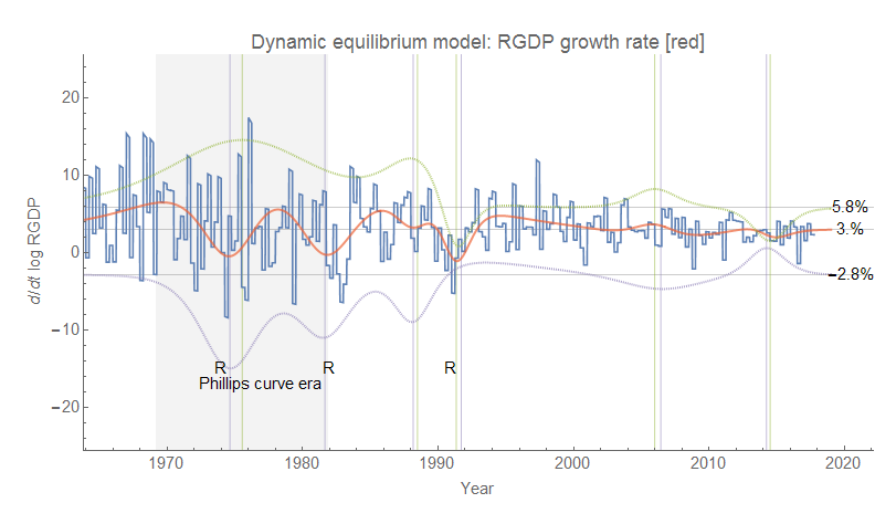
Economic growth in Australia 1960-present

I saw the chart above on Twitter; it made me want to try this analysis using the dynamic information equilibrium model for Australia to see if I could understand the near constant decline in RGDP growth since the early 2000s because it looked very odd from a dynamic equilibrium standpoint. The data I have from FRED for Australia is a bit noisier than the US and UK data so there is the oddity that the model sees the Great Recession as more of a statistical fluctuation than a shock. Here are the models of NGDP and the GDP deflator (click for full resolution):

The dynamic equilibria are 5.8% NGDP growth and 2.8% inflation, resulting in 3%. The demographic shift (discussed below) is highlighted in gray. And here is how they combine as RGDP growth (click for full resolution):

Overall the picture for Australia is approximately the same as for the US and UK: a "Phillips curve era" accompanied by a demographic transition in the mid-to-late 1970s and a more recent era with sparser shocks. I hesitate to give it the same "asset bubble era" label I gave the US and UK because it seems more associated with the "commodity boom" of the 2000s (centered in 2006). There was also a major (nominal) commodities bust centered in 2014, but as it was accompanied by a nearly equal negative shock to inflation it turns out to be a wash in RGDP. In fact both shocks in the post-Phillips curve era effectively combine to create a slow steady decline in RGDP. Here is the dynamic equilibrium model version of the 10-year average RGDP growth graph at the top of this post (click for full resolution):

While the forecast looks a bit strange, it is entirely due to the backward-looking 10 year average (which also makes the 10 year average growth rate higher than the continuously compounded rate about at 3.6%) and in the continuously compounded rate of change we have a simple return to about 3% RGDP growth following the "commodity bust".

Australia is frequenty noted for its long recession-free streak following its early 90s recession (which in fact has almost the exact same structure as the "Lawson boom" — and subsequent bust — in the UK data), with some attributing it to effective monetary policy. I'd attribute it to the high rate of NGDP and RGDP growth (likely stemming from a high rate of population growth, about double the US) that makes even large negative shocks like the Great Recession insufficient to generate more than a single quarter of negative growth (it's effectively interpreted by the model as the ending of the "commodity boom" than its own "shock"). But also the shocks to nominal growth and inflation are both broader and more correlated for Australia resulting in less jagged RGDP growth (which tends to be associated with recessions). This correlation may well be due to the fact that the nominal growth is associated with commodities rather than financial and/or housing asset bubbles in the UK and US (Minsky!). Although housing prices appear to have been rising in Australia (only to begin to decelerate more recently), there does not appear to be a separate "housing bubble" effect readily visible in the data — maybe housing prices were associated with the commodities boom rather than an independent phenomenon (for US readers, think North Dakota housing prices in the 2010s rather than Florida/Arizona in the 2000s)?

But the broad themes here are similar to the US and UK: a big demographic shift has ended (and with it, high growth), and we've entered an era of booms and busts and more moderate growth.

Dynamic equilibrium model: fertility as a leading indicator

A new NBER working paper titled Is fertility a leading economic indicator? by Kasey Buckles, Daniel Hungerman, and Steven Lugauer looks at birth data to show that conceptions (in the graph at the top of the page) are a leading indicator of recessions. Their abstract:

Many papers show that aggregate fertility is pro-cyclical over the business cycle. In this paper we do something else: using data on more than 100 million births and focusing on within-year changes in fertility, we show that for recent recessions in the United States, the growth rate for conceptions begins to fall several quarters prior to economic decline. Our findings suggest that fertility behavior is more forward-looking and sensitive to changes in short-run expectations about the economy than previously thought.

I tried to look at the data using the dynamic information equilibrium model; the details of the model are in my paper [1] where I also looked at JOLTS data as providing a leading indicator of recessions. The model turns out to be a pretty decent description of the data:

And it is a leading indicator, beating out JOLTS data by several months (an economic "seismograph" per here) [2]:

Click for the full resolution image. The interesting thing to me is that a human social factor is a leading indicator with a greater lead time than economic factors (like the number of hires or job openings). This points to recession as a predominantly social phenomenon, not economic, being viable hypothesis. There could well be other economic phenomena with longer lead times (I could see e.g. housing coming first in the decision process of having a child [3]), and it could therefore be more of a mixture of social and economic factors. But the big takeaway is that a recession is a complex process that involves the interaction of many variables over the course of years before the thing that gets called an "NBER recession" is said to start.

...

Update 1 May 2018

The conceptions indicator appears to lead the shock to the Case-Shiller index (click to expand):

...

Footnotes:

[1] The information equilibrium model has a particularly clear interpretation here as "male event" and a "female event" meeting in a "conception event" in physical state space.

[2] C = conceptions, HIR = JOLTS hires, JOR = JOLTS job openings, QUR = JOLTS quits, U = unemployment rate, W = wage growth, CLF = Civilian Labor Force participation rate

[3] The actual mix of factors might also depend strongly on the social institutions of the country in question — the US has particularly stingy maternal/paternal leave provisions and therefore a fall in conceptions might not lead recessions in e.g. France which has much more parent-friendly policies.

Shock cluster analysis and some new visualizations

As part of my attempt to rewrite the macroeconomic history of the United States [1], I've been looking at all of the dynamic information equilibrium model "seismograms" I can. I decided to try some machine learning algorithms to see if there's anything to be extracted. But first, I did some simple clustering using the DBSCAN algorithm. I used only the shock centers (i.e. time) and tried both values (i.e. the years like 1977 or 2008) as well as differences (i.e. the time between shocks like 4 years). The former only seemed to cluster the vectors based on length which is an artifact of the available data. The latter did a bit better [2] and found the following groupings:

For the label definitions, see [3]. In this result, GNP, Case-Shiller housing index, and AMB are all on their own. I believe the JOLTS measures were associated with the CLF measures simply because they were too short — if more JOLTS data was available they'd probably be placed with the unemployment rate. But the most interesting clusters were #2 and #3 which associated NGDP with women's EPOP and the unemployment rate with men's EPOP. This is part of the story about women entering the workforce as a driving factor in growth I've been telling (while men in the workforce are basically a cyclical component).

I've also been trying to come up with a better way to visualize the information — the solid bars (see footnote [1]) do nothing to indicate the relative magnitude of the shocks and only show one measure of the duration (using the width parameter). Here's a first attempt at a "continuous" visualization that also includes magnitude (relative to each individual measure):

In this color scheme, blue are positive (or "good") shocks which red are negative (or "bad") shocks. Inflation is categorized as "good" here. The "beige" regions are where the model is following the dynamic information equilibrium. The demographic shift of women entering the labor force (CLF W) can be seen to precede most of the other macroeconomic measures (NGDP, DEF, etc).

This selection shows the fading Phillips curve (shocks to employment coming alongside falling inflation — the red bands in U following on the falling side the blue bands in DEF fading out by the 2000s) best, with peak "Phillips curve" right in the middle of the shock to women's employment-population ratio:

It also shows how after the demographic shock to women's EPOP, it becomes correlated with men's EPOP (which is correlated with the unemployment rate).

...

Footnotes:

[1] This is part of a longer-term project of self-deprecating hubris. Here's the diagram so far (click for the actual higher resolution version):

[2] "Seismograms" of the clusters:

[3] Legend

GNP = Gross National Produc
NGDP = Nominal Gross Domestic Product
W = Wage growth
EPOP W (M) = Employment population ratio for Women (Men)
SP500 = S&P 500 stock index
U = Unemployment rate
Case-Shiller = Case-Shiller housing price index
CPI (C-S) (cycle) = Consumer price index (Case-Shiller data) (cyclical component)
PCE (cycle) = Personal Consumption Expenditures price index (cyclical component)
HIR, JOR, QUR = JOLTS hire, job opening, and quit rates
CLF W (M) = Civilian Labor Force level for Women (Men)
NGDP/L = Nominal GDP divided by total nonfarm employment
MICH = Michigan inflation expectations
AMB = St. Louis Adjusted Monetary Base
DEF = GDP deflator
CLF part= CLF participation rate

Cyclical component here means that the resolution of the search for shocks was higher (bandwidth of the kernel smoother was smaller). You can interpret these as fluctuations on top of the broad shocks in the low resolution CPI and PCE measures. Since the old "seismograms" don't include magnitude, it is hard to tell that the magnitude of the cyclical CPI/PCE is consistent with the broad shock measure (the largest cyclical shocks happen in the middle of the broad shocks, with the earlier and later ones being much smaller — see the continuous versions above).

Forecast performance of a quantity theory of labor

One of the dynamic information equilibrium model forecasts I've been tracking on the order of a year now to measure its performance is what I call the "N/L" or "NGDP/L" model [1] (specifically FRED GDP, i.e. nominal GDP, divided by FRED PAYEMS, i.e. total nonfarm payrolls). Revised GDP data came out today, so I thought it'd be a good time to check back in with the model [2]:

One way to think about this is as a measure of nominal productivity. We are coming out of the aftermath of the shock to the labor force following the great recession, so we can see a gradual increase back towards the long-run equilibrium.

If we use this dynamic equilibrium model instead of NGDP alone as the shocks, we can see in a history "seismograph" that this measure basically coincides with the inflation measures.

There's a good reason for this: this is effectively a model of Okun's law (as described here) if we identify the "abstract price" with the price level P:

$$
P \equiv \frac{dNGDP}{dL} = k \; \frac{NGDP}{L}
$$

which can be rearranged

$$
\begin{align}
L & = k \; \frac{NGDP}{P} \equiv RGDP\\
\frac{d}{dt} \log L & = \frac{d}{dt} \log RGDP
\end{align}
$$

to show changes in employment (and therefore unemployment) are directly related to changes in real GDP.

...

Footnotes

[1] Also, the "quantity theory of labor" per the title because the model implies log NGDP ~ k log L.

[2] Here is the complete model:

Women in the workforce and the Solow paradox

Paddy Carter sent me a link on Twitter to a study [pdf] using a different model that came to conclusions similar to the view I've been expressing on this blog:

The increase in female employment and participation rates is one of the most dramatic changes to have taken place in the economy during the last century.

From their conclusions:

Furthermore, the unexplained portion [of the rise in women's employment] is quite large and positive; in other words, for cohorts born before 1955, the simulations overpredict female employment and for more recent cohorts, underpredict it. Therefore, there must have been other changes taking place among married women by cohort. We have shown above that it is consistent with the model to claim that technological progress in household production or a change in social norms has brought down the costs of working outside the home.

As part of my continuing series of dynamic information equilibrium "seismograms" (previously here), I put together another version of the story of women entering the workforce [1] as a driver of dramatic changes in the economy:

A big lesson is about causality. The positive shock to the level of women in the labor force precedes a (smaller relative) shock to the level of men in the labor force, both of which precede shocks to output and finally inflation (both CPI and PCE shown). Women entering the workforce caused a general economic boom — which drew additional men into the workforce and increased output and prices.

In the study linked above, the authors speculate that some of the effect was due to "technological progress in household production" (e.g. household labor-saving devices like washing machines and dishwashers) which made me think of the 'Solow paradox' ("You can see the computer age everywhere but in the productivity statistics."). What if the reason that household technology shows up in the economy is because household technology enabled more people to enter the labor force, while computers were mostly used by people already in the labor force [2]? This idea can be taken a step further to suggest that maybe the high GDP growth and inflation of the 1970s was due to the fact that a significant fraction of work that isn't counted in GDP statistics (household production) was automated allowing people to participate in work that was counted in GDP. That is to say that if household production was counted in GDP, it is possible that there might not have been a "great inflation".

This is of course speculative. However it is a good "thought experiment" to keep in mind to keep you from assuming that GDP is some ideal measure and remind you that the "events" that appear in the GDP data may well be artefacts of the measurement methodology [3].

...

Update

Diane Coyle makes the case [pdf] for the possibility I mention in footnote [2]: transition to more "digital production" behind recent low productivity.

...

Update 28 February 2018

Commenter Anti below mentions inflation expectations, so I thought I'd add the dynamic information equilibrium model of the price level implied by the University of Michigan inflation expectations data [4]. I've added the result to the macroeconomic seismogram:

Note that shock to inflation expectations follows the shock to measured inflation (making a simple backward-looking martingale a plausible model).

...

Footnotes

[1] Here are the CLF models for men and women:

The NGDP model is from here; the inflation models were used in my first history seismogram.

[2] This brings up the question of whether current home production that isn't counted in GDP — much of which is done on computers — is behind the recent "low growth" of a lot of developed economies.

[3] And even the economic system as households (as well as firms) are typically more like miniature centrally planned economies.

[4] The model fit is pretty good (dynamic equilibrium is α = 0.03, or basically 3% inflation):

Dynamic equilibrium in wage growth

I saw some data from the Atlanta Fed [1] on wage growth that looked remarkably suitable for a dynamic information equilibrium model (also described in my recent paper). One of the interesting things here is that it is a dynamic equilibrium between wages ($W$) and the rate of change of wages ($dW/dt$) so that we have the model $dW/dt \rightleftarrows W$:

$$
\frac{d}{dt} \log \frac{d}{dt} \log W = \frac{d}{dt} \log \frac{dW/dt}{W} \approx \gamma + \sigma_{i} (t)
$$

where $\gamma$ is the dynamic equilibrium growth rate and $\sigma_{i} (t)$ represents a series of shocks. This model works remarkably well:

The shock transitions are in 1992.0, 2002.4, 2009.4, and 2014.7 which all follow the related shock to unemployment. A negative shock to employment drives down wage growth (who knew?), but it also appears that wage growth has a tendency to increase at about 4.2% per year [2] unless there is a positive shock to employment (such as in 2014) when it can increase faster. The most recent downturn in the data is possibly consistent with the JOLTS leading indicators showing a deviation, however since the wage growth data seems to lag recessions it is more likely that this is a measurement/noise fluctuation.

I added the wage growth series to the labor market "seismogram" collection, and we can see a fall in wage growth typically follows a recession:

...

Update 20 March 2021

It's not groundbreaking, but I should add that since $W \rightleftarrows NGDP$, the model is basically (by the transitive property of information equilibrium) that increases in NGDP are informationally equivalent to increases in the rate of growth of wages — a growing economy opens the opportunity set for wage growth.

At least until this happens.

(I've felt that the $\frac{dW}{dt} \rightleftarrows W$ formulation was a bit abstract, but realized I've never updated the post with how I thought about it in a more concrete way.)

...

Footnotes:

[1] The time series is broken before 1997, but data goes back to 1983 in the source material. I included data back to 1987. However the data prior the 1991 recession does not have the complete 1980s recession(s), so the fit to that recession shock would be highly uncertain and so I left it out.

[2] Wage growth it typically around 3.0% lately, so a 4.2% increase in that rate would mean that after a year wage growth would be about 3.1% and after 2 years about 3.3% in the absence of shocks.

Are interest rates inexplicably high?

The interest rate model of the long and short term interest rates are predicting average interest rates below the current observed rates. For example in this forecast:

Now the actual forecast is for the average trend of monthly rates and I'm showing actual daily interest rate data, so we can expect to see occasional deviations even if the model is working correctly.

But how can we tell the difference between some expected theoretical error and a deviation? I decided to look at the elevated recent data in the light of the models' typical error. In the case of the long rate above, we're in the normal range:

The short rate is on a significant deviation:

However these errors basically assume that the model error is roughly constant in percentage (i.e. a 10% error means 100 basis point error on a 10% interest rate while a 10% error means a 10 basis point error on a 1% interest rate). This is definitely not true because the data is reported only to the nearest basis point, but the finite precision effect should only come into play near log(0.01) ~ -4.6. This error is possibly due to the Federal Reserve's implied precision of 25 basis points where log(0.25) ~ -1.4. Since the Fed doesn't make changes of less than a quarter basis point, and the short rate typically sticks close to the Fed funds rate, we'd expect data near or below log(0.25) as shown on the graph to have larger error than points above log(0.25).

I don't see any particular reason to abandon these models without a more significant deviation.